Data ETL • WADashboard

This vignette documents the steps to ingest model output files (in CSV and NetCDF format) for use in the dashboard.

This ETL was validated against two analyses received from IWMI scientists, one for Mali (Niger river basin), and another for Kenya (Mara river basin). The water accounting models are written in Python and the code repositories are on GitHub (e.g. WAPORWA notebooks for the Mali analysis).

The results of the WA+ balances consist in time-series of constructed hydrological variables – the time steps can vary (dekadal, monthly, seasonal, yearly steps). The series are either gridded (NetCDF) or aggregated over an entire zone of interest (CSV output files). The modeled variables are further enriched to construct visual balances (or “Sheets”) that represent key water availability, use and management indicators over time.

The WA+ modeling approach can vary slightly across use cases (different temporal extent, number of sub-basins, different flow units, different mix of input layers and output variables). To the extent possible this ETL intends to produce a generalized data model.

The steps outlined below serve as a blueprint for a generic data_etl() method included in this package (refer to the method’s documentation for more details, esp. how to ingest additional result sets). The objective is to generate a data cube suitable for online analytics.

# Location of model output datasets
dir <- getOption("wa.data")

# Plot defaults
th <- function(...) theme(
  legend.position = "none",
  panel.spacing.y = unit(0, "lines"),
  strip.text.y = element_text(size=7, angle=0, hjust=0),
  strip.background = element_blank(),
  axis.text.y = element_blank(),
  axis.title.y = element_blank(),
  axis.ticks.y = element_blank(),
  panel.border = element_blank(),
  panel.grid = element_blank(),
  panel.background = element_blank(),
  ...)

Basin-level Aggregates (CSV files)

We start below by inventorying all basin-level variables contained in the modeled CSV files.

# List all output CSV
data <- list(
  ken = file.path(dir, "./ken/hydroloop_results/csv"),
  mli = file.path(dir, "/mli/csv_km3")
) %>%
  lapply(list.files, pattern="*.csv", recursive=TRUE, full.names=TRUE) %>%
  lapply(data.table) %>%
  rbindlist(idcol="iso3", use.names=TRUE, fill=TRUE) %>%
  setnames("V1", "path")

# Extract timestamps and sheet codes from file names
data[, `:=`(
  file = basename(path)
)][, `:=`(
  year = str_extract(file, "_[0-9]{4}") %>% str_sub(2,5) %>% as.integer(),
  month = str_extract(file, "[0-9]{4}_[0-9]{1,2}") %>% str_sub(6,7) %>% as.integer(),
  sheet = str_extract(tolower(file), "sheet[0-9]{1}") 
)] %>% setorder(iso3, sheet, year, month, na.last=TRUE)

# Append flow units (typically km3 or MCM, will need to be specified manually)
data[, unit := fcase(
  iso3=="mli", "km3",
  iso3=="ken", "km3"
)]

We have 8 yearly water balances for Mali (Sheet #1 variables), 15 yearly balances for Kenya (across 6 sheets), as well as monthly and seasonal breakdowns.

data[iso3=="mli", .(iso3, file, sheet, year, month)] %>% 
  paged_table()

ABCDEFGHIJ0123456789

iso3 <chr>	file <chr>	sheet <chr>	year <int>	month <int>
mli	Sheet1_2010.csv	sheet1	2010	NA
mli	Sheet1_2011.csv	sheet1	2011	NA
mli	Sheet1_2012.csv	sheet1	2012	NA
mli	Sheet1_2013.csv	sheet1	2013	NA
mli	Sheet1_2014.csv	sheet1	2014	NA
mli	Sheet1_2015.csv	sheet1	2015	NA
mli	Sheet1_2016.csv	sheet1	2016	NA
mli	Sheet1_2017.csv	sheet1	2017	NA

data[iso3=="ken" & !is.na(year) & is.na(month), .(iso3, file, sheet, year, month)] %>% 
  paged_table()

ABCDEFGHIJ0123456789

iso3 <chr>	file <chr>	sheet <chr>	year <int>	month <int>
ken	sheet1_2003.csv	sheet1	2003	NA
ken	sheet1_2004.csv	sheet1	2004	NA
ken	sheet1_2005.csv	sheet1	2005	NA
ken	sheet1_2006.csv	sheet1	2006	NA
ken	sheet1_2007.csv	sheet1	2007	NA
ken	sheet1_2008.csv	sheet1	2008	NA
ken	sheet1_2009.csv	sheet1	2009	NA
ken	sheet1_2010.csv	sheet1	2010	NA
ken	sheet1_2011.csv	sheet1	2011	NA
ken	sheet1_2012.csv	sheet1	2012	NA

data[iso3=="ken" & !is.na(month), .(iso3, file, sheet, year, month)] %>% 
  paged_table()

ABCDEFGHIJ0123456789

iso3 <chr>	file <chr>	sheet <chr>	year <int>	month <int>
ken	sheet1_2003_1.csv	sheet1	2003	1
ken	sheet1_2003_2.csv	sheet1	2003	2
ken	sheet1_2003_3.csv	sheet1	2003	3
ken	sheet1_2003_4.csv	sheet1	2003	4
ken	sheet1_2003_5.csv	sheet1	2003	5
ken	sheet1_2003_6.csv	sheet1	2003	6
ken	sheet1_2003_7.csv	sheet1	2003	7
ken	sheet1_2003_8.csv	sheet1	2003	8
ken	sheet1_2003_9.csv	sheet1	2003	9
ken	sheet1_2003_10.csv	sheet1	2003	10

The Kenya analysis also includes yearly, seasonal, and monthly time-series for an additional 57 variables:

data[iso3=="ken" & is.na(year) & is.na(month), .(iso3, file, sheet, year, month)] %>% 
  paged_table()

ABCDEFGHIJ0123456789

iso3 <chr>	file <chr>	sheet <chr>	year <int>	month <int>
ken	sheet1_basin_etincr_monthly.csv	sheet1	NA	NA
ken	sheet1_basin_etrain_monthly.csv	sheet1	NA	NA
ken	sheet1_basin_p_monthly.csv	sheet1	NA	NA
ken	sheet2_lu_e_monthly.csv	sheet2	NA	NA
ken	sheet2_lu_et_monthly.csv	sheet2	NA	NA
ken	sheet2_lu_i_monthly.csv	sheet2	NA	NA
ken	sheet2_lu_t_monthly.csv	sheet2	NA	NA
ken	sheet3_35.0_et_depth_season.csv	sheet3	NA	NA
ken	sheet3_35.0_et_depth_yearly.csv	sheet3	NA	NA
ken	sheet3_35.0_et_season.csv	sheet3	NA	NA

Variable Inspection

We also need to validate naming conventions and units for all output variables, so we continue by inspecting individual files starting with Mali.

Sheet #1

f <- data[iso3=="mli"]

mli <- lapply(1:nrow(f), function(x) fread(f[x, path])[, `:=`(
  iso3 = f[x, iso3],
  sheet = f[x, sheet],
  year = f[x, year]
)]) %>% rbindlist()

setnames(mli, tolower(names(mli)))
mli %>% paged_table(options=list(max.print=300))

ABCDEFGHIJ0123456789

class <chr>	subclass <chr>	variable <chr>	value <dbl>	iso3 <chr>	sheet <chr>	year <int>
INFLOW	PRECIPITATION	Rainfall	434.99	mli	sheet1	2010
INFLOW	PRECIPITATION	Snowfall	0.00	mli	sheet1	2010
INFLOW	PRECIPITATION	Precipitation recycling	0.00	mli	sheet1	2010
INFLOW	SURFACE WATER	Main riverstem	0.00	mli	sheet1	2010
INFLOW	SURFACE WATER	Tributaries	0.00	mli	sheet1	2010
INFLOW	SURFACE WATER	Utilized surface water	0.00	mli	sheet1	2010
INFLOW	SURFACE WATER	Flood	0.00	mli	sheet1	2010
INFLOW	GROUNDWATER	Natural	0.00	mli	sheet1	2010
INFLOW	GROUNDWATER	Utilized	0.00	mli	sheet1	2010
INFLOW	OTHER	Desalinized	0.00	mli	sheet1	2010

Output for Sheet #1 include 34 unique variables categorized into class and subclass. The naming is consistent across years.

mli %>% 
  ggplot() +
  geom_line(aes(year, value, color=paste(class, subclass))) +
  facet_grid(paste(class, subclass, variable)~., scales="free_y") +
  th() +
  labs(x=NULL, y=NULL) +
  ggtitle("WA+ Sheet 1 Variables - Mali, 2009 to 2016")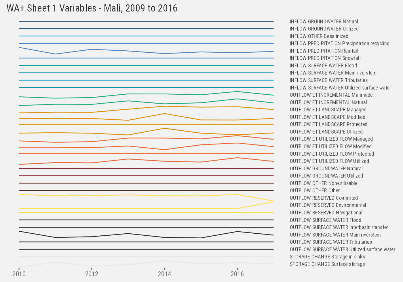

Similarly we look at Kenya’s monthly time-series. First at Sheet #1 variables:

f <- data[iso3=="ken" & !is.na(month) & !is.na(year) & sheet=="sheet1"]
ken_1 <- lapply(1:nrow(f), function(x) fread(f[x, path])[, `:=`(
  iso3 = f[x, iso3],
  sheet = f[x, sheet],
  year = f[x, year],
  month = f[x, month]
)]) %>% rbindlist()

setnames(ken_1, tolower(names(ken_1)))
ken_1 %>% paged_table(options=list(max.print=300))

ABCDEFGHIJ0123456789

class <chr>	subclass <chr>	variable <chr>	value <dbl>	iso3 <chr>	sheet <chr>	year <int>	month <int>
INFLOW	PRECIPITATION	Rainfall	6.508760e-01	ken	sheet1	2003	1
INFLOW	PRECIPITATION	Snowfall	0.000000e+00	ken	sheet1	2003	1
INFLOW	PRECIPITATION	Precipitation recycling	0.000000e+00	ken	sheet1	2003	1
INFLOW	SURFACE WATER	Main riverstem	0.000000e+00	ken	sheet1	2003	1
INFLOW	SURFACE WATER	Tributaries	0.000000e+00	ken	sheet1	2003	1
INFLOW	SURFACE WATER	Utilized surface water	0.000000e+00	ken	sheet1	2003	1
INFLOW	SURFACE WATER	Flood	0.000000e+00	ken	sheet1	2003	1
INFLOW	GROUNDWATER	Natural	0.000000e+00	ken	sheet1	2003	1
INFLOW	GROUNDWATER	Utilized	0.000000e+00	ken	sheet1	2003	1
INFLOW	OTHER	Desalinized	0.000000e+00	ken	sheet1	2003	1

ken_1 %>% 
  ggplot() +
  geom_line(aes(as.Date(paste(year, month, 1), "%Y %m %d"), value, color=subclass)) +
  facet_grid(paste(class, subclass, variable)~., scales="free_y") +
  th() +
  labs(x=NULL, y=NULL) +
  ggtitle("WA+ Sheet 1 Variables - Kenya, 2003 to 2017")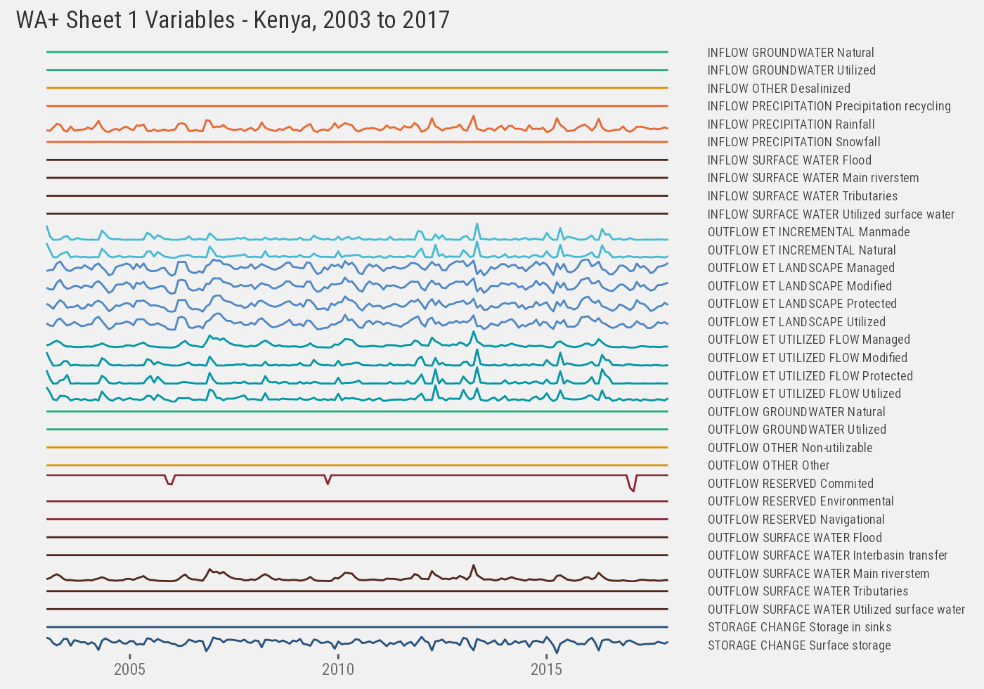

Sheet #2

Then we extract Sheet #2 variables (this is a breakdown of evapotranspiration by land use classes):

f <- data[iso3=="ken" & !is.na(month) & !is.na(year) & sheet=="sheet2"]
ken_2 <- lapply(1:nrow(f), function(x) fread(f[x, path])[, `:=`(
  iso3 = f[x, iso3],
  sheet = f[x, sheet],
  year = f[x, year],
  month = f[x, month]
)]) %>% rbindlist()

setnames(ken_2, tolower(names(ken_2)))
ken_2 %>% paged_table(options=list(max.print=300))

ABCDEFGHIJ0123456789

land_use <chr>	class <chr>	transpiration <dbl>	water <dbl>	soil <dbl>	interception <dbl>	agriculture <dbl>	environment <dbl>
PROTECTED	Forest	3.392319e-02	0.000000e+00	6.037666e-03	4.300275e-03	0.000000e+00	3.396673e-02
PROTECTED	Shrubland	4.284608e-02	0.000000e+00	8.178200e-03	5.136607e-03	0.000000e+00	4.337064e-02
PROTECTED	Natural grasslands	1.228219e-01	0.000000e+00	2.352691e-02	1.512350e-02	0.000000e+00	1.243965e-01
PROTECTED	Natural water bodies	0.000000e+00	0.000000e+00	0.000000e+00	0.000000e+00	0.000000e+00	0.000000e+00
PROTECTED	Wetlands	5.551789e-05	0.000000e+00	8.703940e-06	5.529845e-06	0.000000e+00	5.458855e-05
PROTECTED	Glaciers	0.000000e+00	0.000000e+00	0.000000e+00	0.000000e+00	0.000000e+00	0.000000e+00
PROTECTED	Others	0.000000e+00	0.000000e+00	0.000000e+00	0.000000e+00	0.000000e+00	0.000000e+00
UTILIZED	Forest	1.189515e-01	0.000000e+00	3.972395e-02	1.701593e-02	5.947573e-03	1.070563e-01
UTILIZED	Shrubland	7.850386e-02	0.000000e+00	1.945468e-02	8.494423e-03	3.925193e-03	6.672828e-02
UTILIZED	Natural grasslands	4.758757e-02	0.000000e+00	1.245738e-02	4.845101e-03	2.855254e-02	1.427627e-02

Each sheet uses a different data structure, but they can be normalized into a “long” format:

# Normalize
ken_2 <- melt(ken_2, id.vars=c("land_use", "class", "iso3", "sheet", "year", "month"),
  variable.factor=FALSE)
# Standardize category names
setnames(ken_2, c("land_use", "class"), c("class", "subclass"))
setorder(ken_2, class, subclass, variable, year, month)

We only plot variables for the first land use class for illustration purposes:

ken_2[class %in% ken_2[, unique(class)][1]] %>% 
  ggplot() +
  geom_line(aes(as.Date(paste(year, month, 1), "%Y %m %d"), value, color=subclass)) +
  facet_grid(paste(class, subclass, variable)~., scales="free_y") +
  th() +
  labs(x=NULL, y=NULL) +
  ggtitle("WA+ Sheet 2 Variables - Kenya, 2003 to 2017")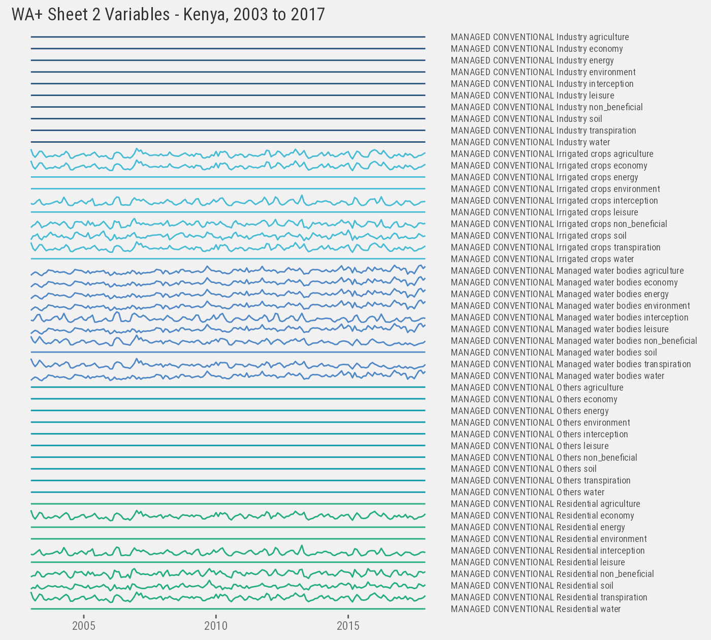

Sheet #3

Similarly we inspect results for Sheet #3 “Agriculture Services”. In the Kenya analysis, variables for Sheet #3 to Sheet #6 are available as yearly, seasonal, and/or monthly time-series (across multiple CSV files).

We (arbitrarily) gather all the seasonal time-series¹:

f <- data[iso3=="ken" & sheet=="sheet3" & 
    str_detect(file, "season") & str_detect(file, "54.0")]
ken_3 <- lapply(1:nrow(f), function(x) fread(f[x, path])[, `:=`(
  iso3 = f[x, iso3],
  sheet = f[x, sheet],
  year = f[x, year],
  month = f[x, month],
  variable = str_replace(f[x, file], "sheet3_54.0_", "") %>% str_replace("_season.csv", "")
)]) %>% rbindlist()

ken_3[, `:=`(
  # Drop counter column
  V1 = NULL,
  # Ensure end of season is last day of month (for consistency with other sheets)
  end_dates = end_dates - 1
)][, `:=`(
  # Encode year/month columns using end of season
  year = year(end_dates),
  month = month(end_dates)
)]

setnames(ken_3, "Seasonal", "value")
setnames(ken_3, c("start_dates", "end_dates"), c("date_start", "date_end"))
setorder(ken_3, variable, year, month)
ken_3 %>% paged_table(options=list(max.print=300))

ABCDEFGHIJ0123456789

date_start <date>	date_end <date>	value <dbl>	iso3 <chr>	sheet <chr>	year <int>	month <int>	variable <chr>
2001-02-01	2001-04-30	NA	ken	sheet3	2001	4	et
2001-10-01	2001-11-30	NA	ken	sheet3	2001	11	et
2002-02-01	2002-04-30	NA	ken	sheet3	2002	4	et
2002-10-01	2002-11-30	NA	ken	sheet3	2002	11	et
2003-02-01	2003-04-30	25124.18204	ken	sheet3	2003	4	et
2003-10-01	2003-11-30	16711.01192	ken	sheet3	2003	11	et
2004-02-01	2004-04-30	27184.55751	ken	sheet3	2004	4	et
2004-10-01	2004-11-30	19600.40617	ken	sheet3	2004	11	et
2005-02-01	2005-04-30	25684.45437	ken	sheet3	2005	4	et
2005-10-01	2005-11-30	17079.47403	ken	sheet3	2005	11	et

Plotting the entire series (6 variables):

ken_3 %>% 
  ggplot() +
  geom_line(aes(as.Date(paste(year, month, 1), "%Y %m %d"), value, color=variable)) +
  facet_grid(variable~., scales="free_y") +
  th() +
  labs(x=NULL, y=NULL) +
  ggtitle("WA+ Sheet 3 Variables - Kenya, 2003 to 2017 (seasonal)")

## Warning: Removed 24 row(s) containing missing values (geom_path).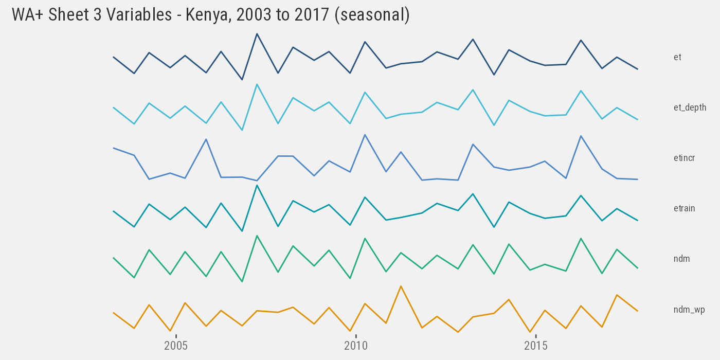

We gather all Sheet #1 to Sheet #3 variables above into a long table format.

cube <- rbind(mli, ken_1, ken_2, ken_3, fill=TRUE)
setcolorder(cube, 
  c("iso3", "sheet", "class", "subclass", "variable", 
    "year", "month", "date_start", "date_end"))

For consistency’s sake, we encode date_start and date_end in all sheets (incl. yearly and monthly variables):

cube[is.na(date_start) & is.na(month), `:=`(
  # yearly series: 1/1 to 12/31
  date_start = as.IDate(paste(year, 1, 1), "%Y %m %d"),
  date_end = as.IDate(paste(year, 12, 31), "%Y %m %d")
)][is.na(date_start) & !is.na(month), `:=`(
  # monthly series: 1/1 to 1/31
  date_start = as.IDate(paste(year, month, 1), "%Y %m %d"),
  date_end = ceiling_date(as.IDate(paste(year, month, 20), "%Y %m %d"), "months") - days(1)
)]

#saveRDS(cube, "./data-raw/rds/data.rds")

The generated data cube includes the following dimensions:

iso3
sheet
class
subclass
variable
year
month
date_start
date_end
value

Data Dictionaries

Another ETL step is required to map the variable codes used in the data files to their visual representation in the WA+ Sheets (SVG designs).

knitr::include_graphics(file.path("./fig", list.files("./vignettes/fig")))

This mapping is embedded in the WA+ print_sheet Python module, (example for Sheet 1 in the WAPORWA repo). Importantly many SVG elements are fields calculated from output variables. We might need to replicate that logic in the dashboard to create dynamic visuals².

Sheet #1

Field mappings are constructed in the table below.

s1 <- fread(system.file("./csv/sheet_1_schema.csv", package="WADashboard")) %>% 
  paged_table()

Formulas for calculated fields are replicated here.

We proceed similarly for Sheet #2 and Sheet #3 mappings.

Sheet #2

Sheet #3

Gridded Variables (netCDF files)

Gridded variables can be used for mapping and/or to calculate sub-basin (or administrative-level) indicators.

Forthcoming…