Section 2 Data Sources and Preprocessing
2.1 Climatic Indicators
Notes on extracting monthly and dekadal climatic indicators from FEWSNET and WorldClim repositories. In the case of FEWSNET all spatial layers are extracted from Jan. 2015 to the latest recorded data point (typically May or June 2017). These data extracts may be used to generate summary statistics over specific planting/growing seasons (for info the effects of biophysical stresses over a typical year are illustrated below).
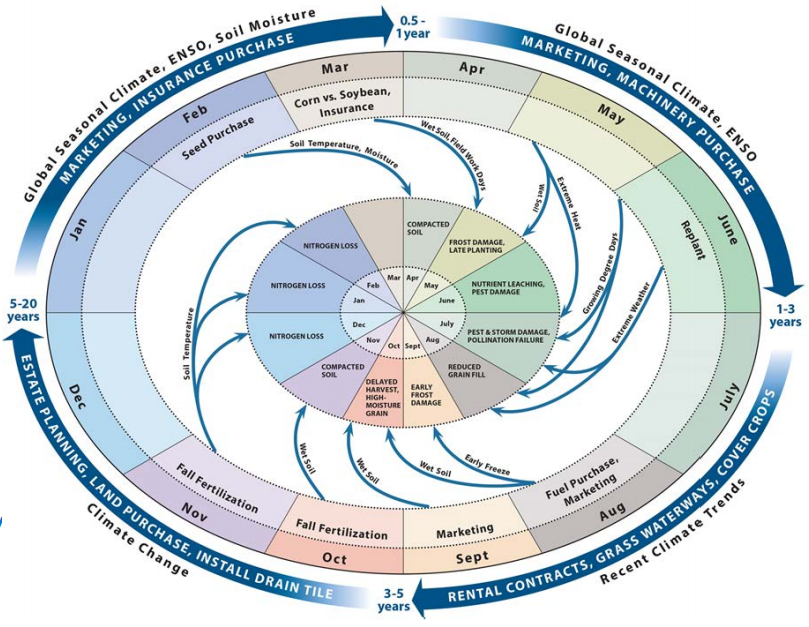
Fig. 2.1: Seasonal Calendar (Haigh et al., 2015)
WorldClim is a repository of long-term climatic time-series for the period 1970-2000 from which to derive 30-year normal baseline data.
2.1.1 FEWSNET
FEWS spatial grids are distributed through multiple channels, primarily USGS and NOAA data portals. There is a series of interactive viewers and tools to explore and download slices of FEWS’ bioclimatic indicators, e.g.:
- http://ewx.chg.ucsb.edu:8080/EWX/index.html
- https://earlywarning.usgs.gov/fews/mapviewer/index.php?region=af
To the author’s knowledge there is no Web service or API to facilitate programmatic access to all of FEWSNET data archives, only public FTP locations1:
FEWS/USGS
https://edcintl.cr.usgs.gov/downloads/sciweb1/shared/fews/web/
Contains RFE2, PET3, ETa4, NDVI5 at different timescales (daily, dekadal, monthly, yearly) and resolutions (usually 1km or lower), and across different regions in Africa.FEWS/NOAA
ftp://ftp.cpc.ncep.noaa.gov/fews/fewsdata/africa
Contains daily ARC26 and RFE7 rainfall estimates for Africa at 10km resolution
In this study all spatial estimates are derived from grids acquired at the following locations:
chirps(monthly, mm, 0.05 degree/~5km) – https://edcintl.cr.usgs.gov/downloads/sciweb1/shared/fews/web/global/monthly/chirps/final/downloads/monthly/
rfe(dekadal, mm, 0.1 degree/~10km) – https://edcintl.cr.usgs.gov/downloads/sciweb1/shared/fews/web/africa/dekadal/rfe/dekadrainfall/downloads/dekadal/
pet(daily, daily mean, mm, 1 degree/~100km) – https://edcintl.cr.usgs.gov/downloads/sciweb1/shared/fews/web/global/daily/pet/downloads/monthly/etaactual ET (dekadal, mm, 0.01 degree/~1km) – https://edcintl.cr.usgs.gov/downloads/sciweb1/shared/fews/web/africa/dekadal/eta/downloads/
et_anomET Anomaly (monthly, percent of median, 0.01 degree/~1km) – https://edcintl.cr.usgs.gov/downloads/sciweb1/shared/fews/web/africa/monthly/eta/anomaly/downloads/
ndvi(dekadal, daily mean, 250m) – https://edcintl.cr.usgs.gov/downloads/sciweb1/shared/fews/web/africa/east/dekadal/emodis/ndvi_c6/temporallysmoothedndvi/downloads/dekadal/
ndvi_anomNDVI Anomaly (dekadal, percent of normal, 250m) – https://edcintl.cr.usgs.gov/downloads/sciweb1/shared/fews/web/africa/east/dekadal/emodis/ndvi_c6/percentofmedian/downloads/
Note that SPEI/SPI (standardized precipitation indices) are not available from FEWS database (see missing downloads at https://edcintl.cr.usgs.gov/downloads/sciweb1/shared/fews/web/africa/dekadal/spi/). An alternative source is SPEIBase v2.4 (2016), but this database does not include the last 2 years 2015-2017 yet and the 0.5 degree resolution is a little coarse for this study.
USGS also warns that the most recent 3 dekadal grids are not always corrected for cloud cover (cloud mask produces misleading zero values).
| Indicator | Periodicity | Resolution | Start | End | Rasters |
|---|---|---|---|---|---|
| chirps | month | 0.050000 | 2015-01-15 | 2017-05-15 | 29 |
| et_anom | month | 0.009652 | 2015-01-15 | 2017-05-15 | 29 |
| eta | dekad | 0.009652 | 2015-01-01 | 2017-06-11 | 89 |
| ndvi_anom_east | dekad | 0.002413 | 2015-01-01 | 2017-06-11 | 89 |
| ndvi_anom_west | dekad | 0.002413 | 2015-01-01 | 2017-06-11 | 89 |
| ndvi_east | dekad | 0.002413 | 2015-01-01 | 2017-06-11 | 89 |
| ndvi_west | dekad | 0.002413 | 2015-01-01 | 2017-06-11 | 89 |
| pet | day | 1.000000 | 2015-01-01 | 2017-06-30 | 912 |
| rfe | dekad | 0.100000 | 2015-01-01 | 2017-06-11 | 89 |
The series of maps below show all FEWSNET indicators (most recent data point) used in this study layered under Nigeria and Kenya’s household locations (after imputation). These maps provide a good perspective of input scale and resolution.
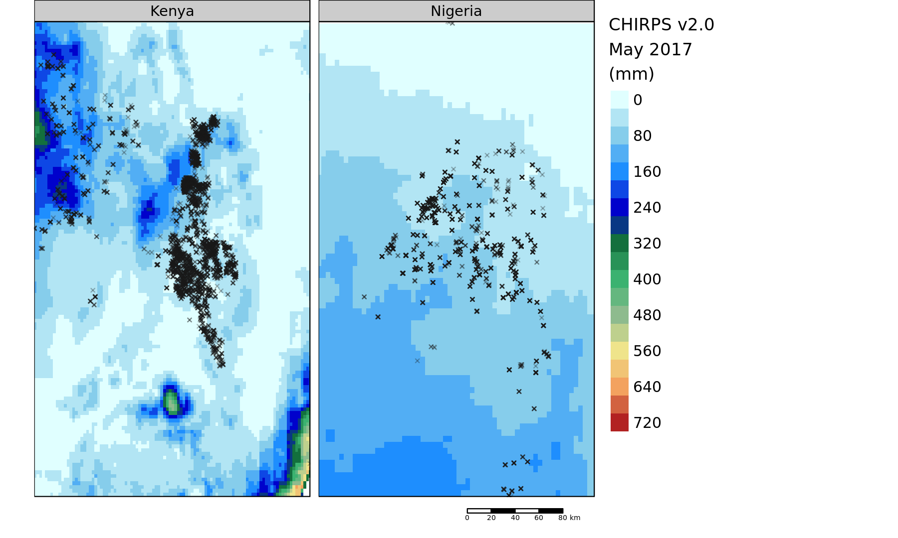
Fig. 2.2: CHIRPS v2.0 (May 2017, mm)
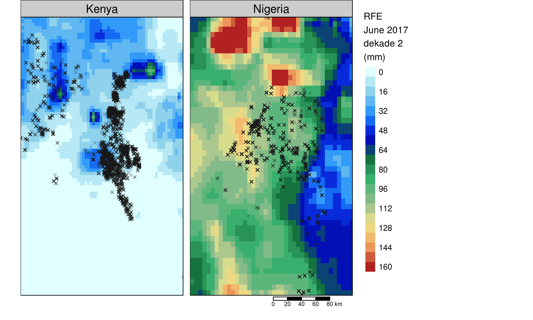
Fig. 2.3: RFE (June 2017, mm)
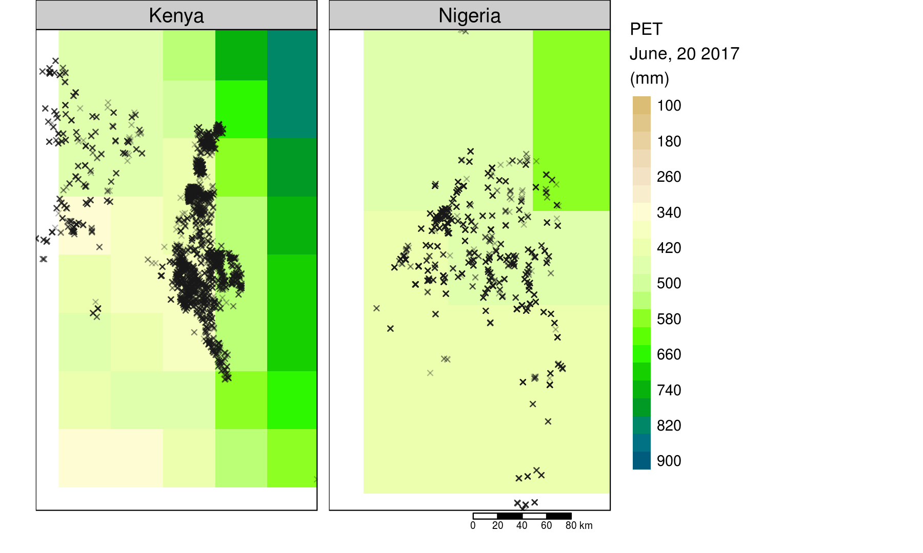
Fig. 2.4: Potential Evapotranspiration (June 30, 2017, mm)
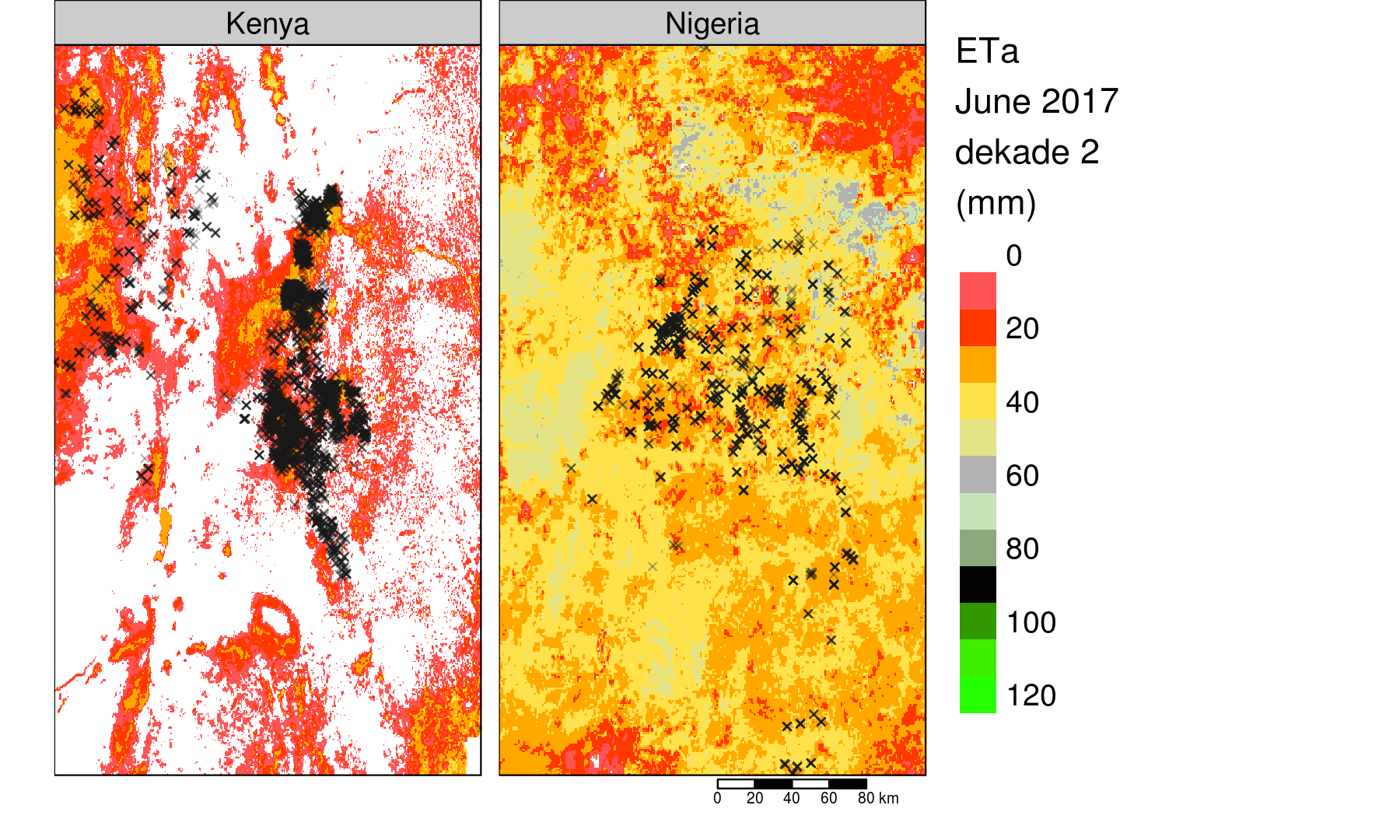
Fig. 2.5: ETa (June 2017, mm)
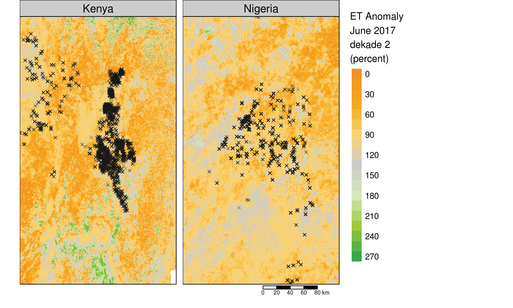
Fig. 2.6: ET Anomaly (June 2017, percent of median)
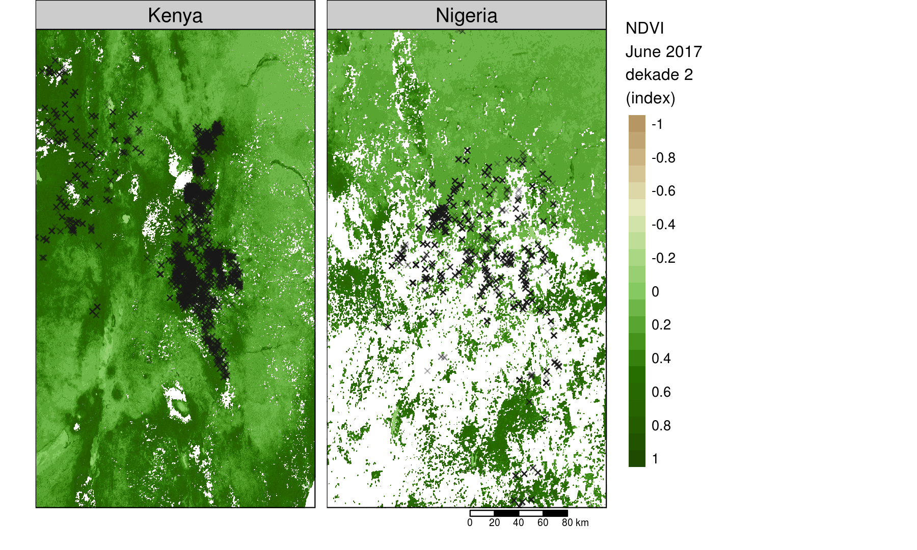
Fig. 2.7: NDVI (June 2017, 0-1 index)
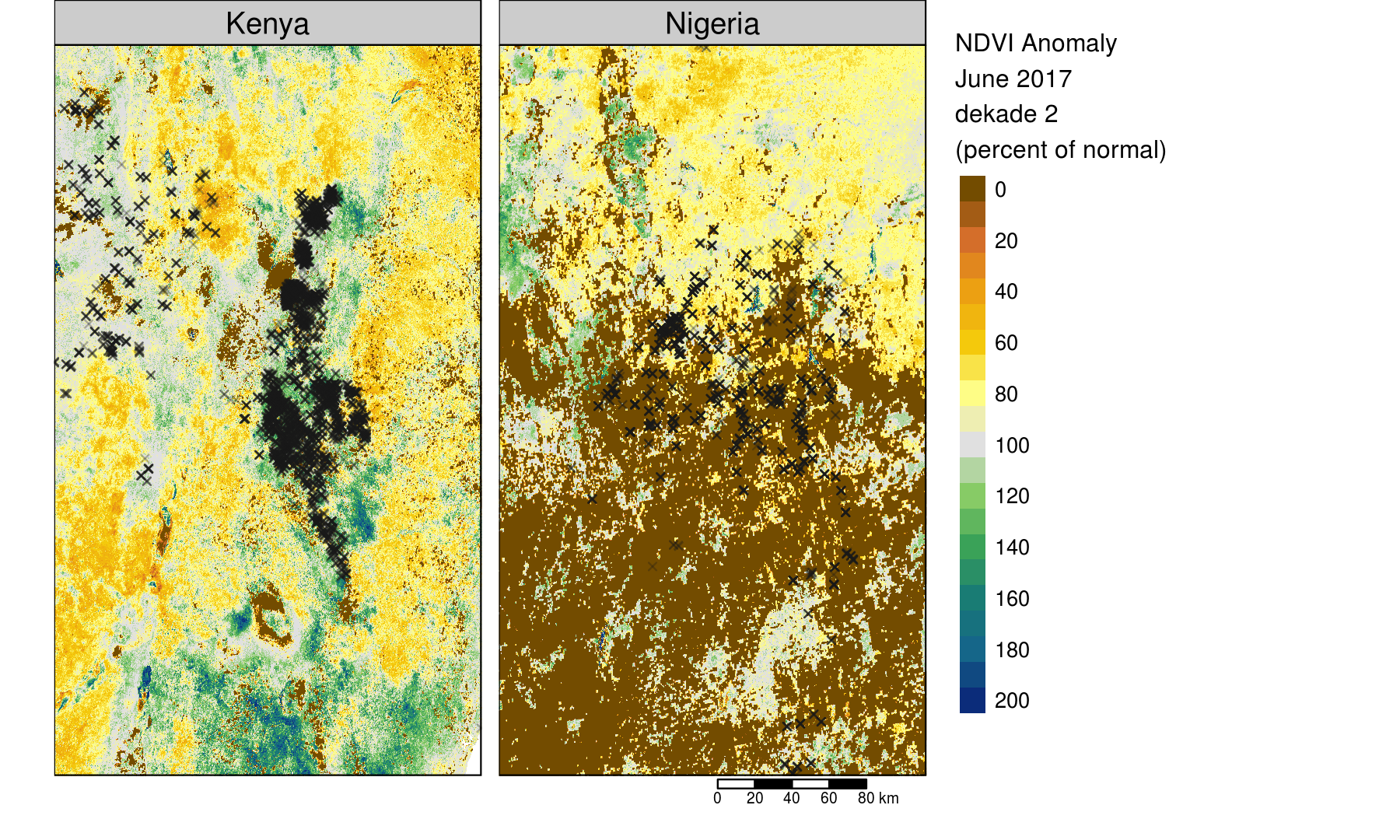
Fig. 2.8: NDVI Anomaly (June 2017, percent of 10-year median 2007-2016)
2.1.2 WorldClim
WorldClim version 2 has long-term average monthly climate data for minimum, mean, and maximum temperature and for precipitation for 1970-2000:
tminminimum temperature (°C)tmaxmaximum temperature (°C)
tavgaverage temperature (°C)precprecipitation (mm)sradsolar radiation (kJ m-2 day-1)windwind speed (m s-1)vaprwater vapor pressure (kPa)
WorldClim also provides a series of 19 long-term bioclimatic variables reflecting annual trends seasonality (annual range in temperature and precipitation) and extreme or limiting environmental factors (temperature of the coldest and warmest month, and precipitation of the wet and dry quarters):
bio1annual mean temperature
bio2mean diurnal range (mean of monthly (max temp - min temp))
bio3isothermality (bio2/bio7) (* 100)
bio4temperature seasonality (standard deviation *100)
bio5max temperature of warmest month
bio6min temperature of coldest month
bio7temperature annual range (bio5-bio6)
bio8mean temperature of wettest quarter
bio9mean temperature of driest quarter
bio10mean temperature of warmest quarter
bio11mean temperature of coldest quarter
bio12annual precipitation
bio13precipitation of wettest month
bio14precipitation of driest month
bio15precipitation seasonality (coefficient of variation)
bio16precipitation of wettest quarter
bio17precipitation of driest quarter
bio18precipitation of warmest quarter
bio19precipitation of coldest quarter
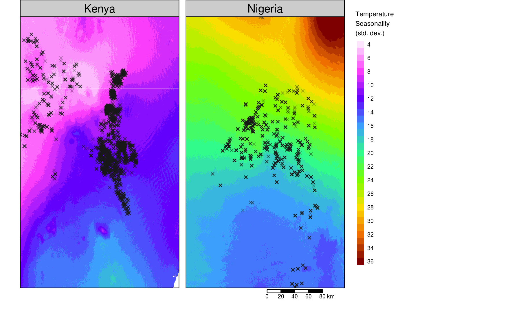
Fig. 2.9: Temperature Seasonality (std. dev., 1970-2000). Source: WorldClim.
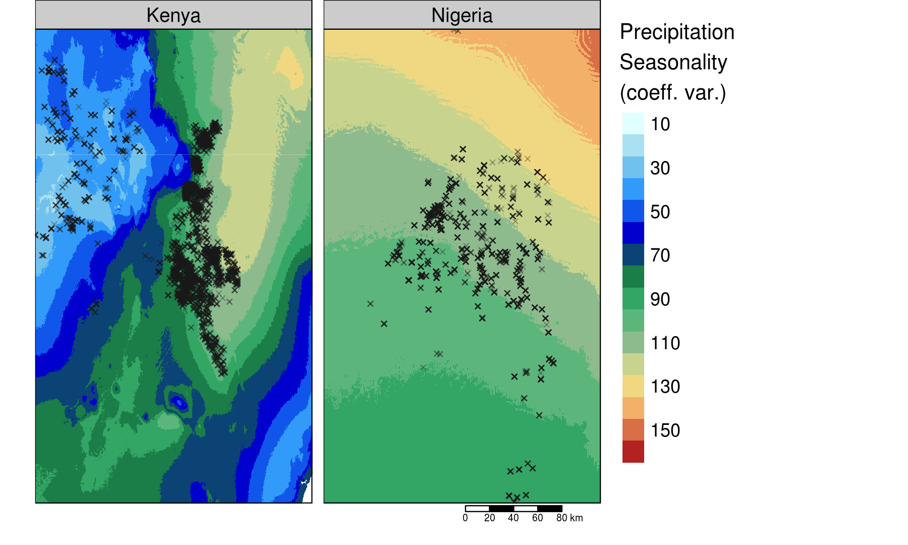
Fig. 2.10: Precipitation Seasonality (coef. var., 1970-2000). Source: WorldClim.
2.1.3 Other Sources
There are other sources of current climatic conditions. They are listed here for reference, but not used.
2.1.3.1 IrriSAT
IrriSAT is a weather based irrigation scheduling service which is used to inform farmers how much water their crop has used and how much how much irrigation they need to apply. Information is produced daily, and can work across large spatial scales. The IrriSAT methodology uses satellite images to determine a Normalized Difference Vegetation Index (NDVI) for each field, from which the plant canopy size can be determined and a specific crop coefficient (Kc) can be estimated.
IrriSAT provides a web API to batch retrieve daily NDVI and Kc at user-specified locations.
irrisat.services.data.cropgrowth()2.1.3.2 aWhere
aWhere is a US for-profit that provides simplified access to current (up to 30 months) global weather conditions at registered field locations. Recently aWhere launched an R client to access their Web APIs. The service is not free (and acccording to their literature it is not meant to collect data for hundred or thousands of point locations). Similar information is available for free from AfSIS and WorldGrids (see below).
2.1.3.3 University of East Anglia CRU TS v4.00
http://browse.ceda.ac.uk/browse/badc/cru/data/cru_ts/cru_ts_4.00/
2.1.3.4 ECMWF ERA5 (2010–2016)
ERA5 is a global atmospheric reanalysis (replacing ERA-Interim). ERA5 Climate reanalysis gives a numerical description of the recent climate, produced by combining models with observations. It contains estimates of atmospheric parameters such as air and soil temperature, pressure and wind at different altitudes, and surface parameters such as rainfall, soil moisture content, sea-surface temperature and wave height. ERA5 provides data at a considerably higher spatial and temporal resolution than its predecessor ERA-Interim: hourly analysis fields are available at a horizontal resolution of 31 km, and on 137 levels from the surface up to around 80 km. Data download is possible through a Web API.
2.2 Drought
Aside from SPEIBase, drought events are also tracked by NASA EONET. NASA EONET API documentation is at https://eonet.sci.gsfc.nasa.gov/docs/v2.1. There’s an R package to query this repository at http://enelmargen.org/nasadata/vignette_v0/. The source of actual drought incidence is also tracked by SEDAC Global Drought Hazard Frequency and Distribution v1 1980-2000), but this source is quite old.
{
"title": "EONET Event Categories",
    "description": "List of all the available event categories in the EONET system",
    "link": "http://eonet.sci.gsfc.nasa.gov/api/v2.1/categories",
    "categories": [
        {
            "id": 6,
            "title": "Drought",
            "link": "http://eonet.sci.gsfc.nasa.gov/api/v2.1/categories/6",
            "description": "Long lasting absence of precipitation affecting agriculture and livestock, and the overall availability of food and water.",
            "layers": "http://eonet.sci.gsfc.nasa.gov/api/v2.1/layers/6"
        }
}
2.3 Soil Characteristics
Data on soil characteristics is obtained from ISRIC and the Africa Soil Information Service (AfSIS). AfSIS generates maps of soil properties at 250m and 1km resolution using legacy soil profile data (from about 12,000 locations in Africa) combined with remote sensing information (climate, land cover, population density, biodiversity, and other covariates). All indicators are available for download at http://geonode.isric.org/ with a web viewer at https://www.soilgrids.org/. The SoilGrids REST API provides support to access data, query and display it, without the need to download the complete grids. REST access to SoilGrids is available through R GSIF package (but too slow to query thousands of points). The following grids were acquired instead:
| Indicator | Label | Resolution | Rasters |
|---|---|---|---|
| ORCDRC_M_sl1_250m_ll | soil organic carbon content at 0 cm | 250m | 1 |
| ORCDRC_M_sl2_250m_ll | soil organic carbon content at 5 cm | 250m | 1 |
| ORCDRC_M_sl3_250m_ll | soil organic carbon content at 15 cm | 250m | 1 |
| ORCDRC_M_sl4_250m_ll | soil organic carbon content at 30 cm | 250m | 1 |
| ORCDRC_M_sl5_250m_ll | soil organic carbon content at 60 cm | 250m | 1 |
| ORCDRC_M_sl6_250m_ll | soil organic carbon content at 100 cm | 250m | 1 |
| ORCDRC_M_sl7_250m_ll | soil organic carbon content at 200 cm | 250m | 1 |
| TAXNWRB_250m_ll | soil class based on the World Reference Base | 250m | 1 |

Fig. 2.11: Dominant Soil Texture. Source: AfSIS 250m.
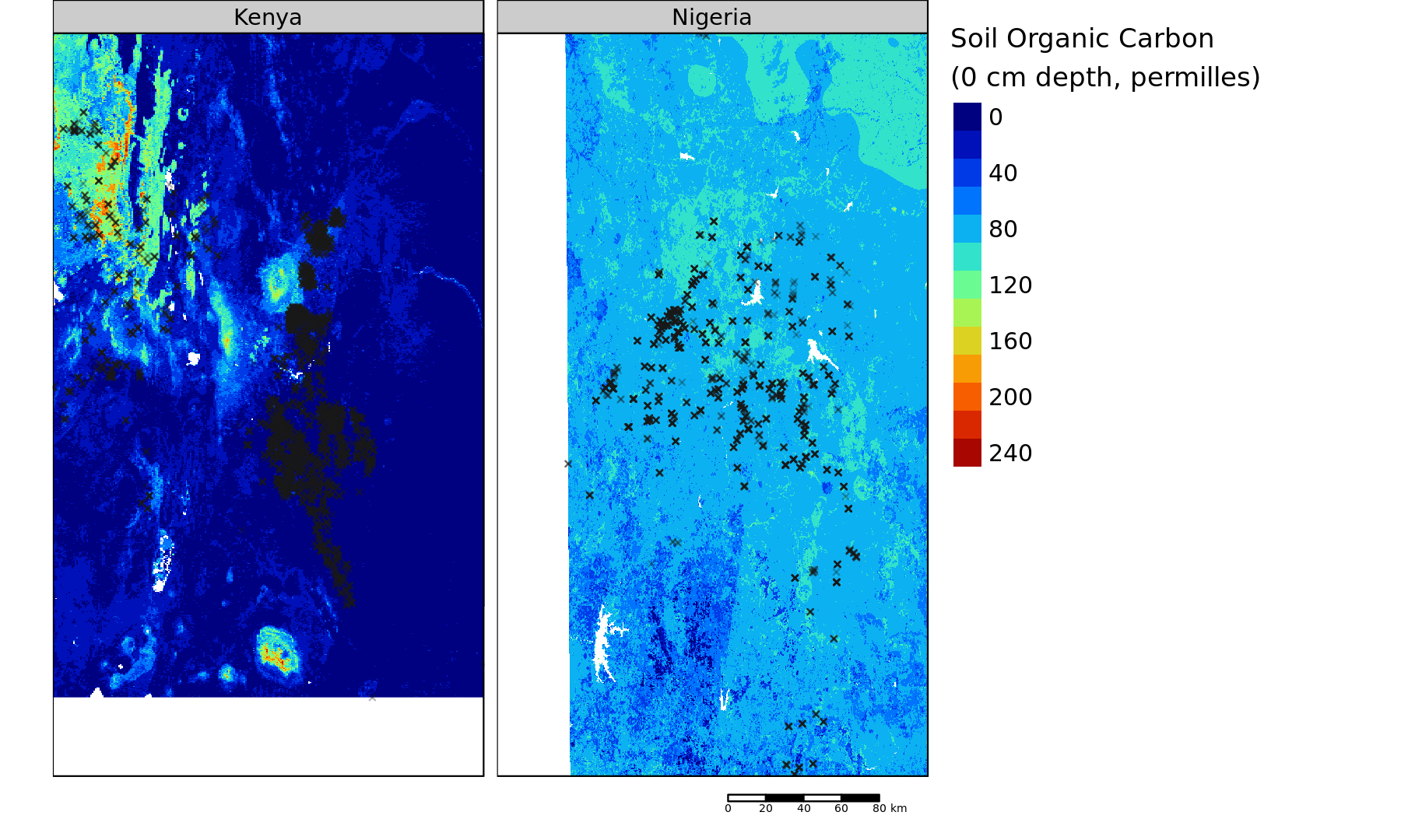
Fig. 2.12: Soil organic Carbon Content (depth 0 cm). Source: SoilGrids 250m.
2.4 Market Access
2.4.1 IFPRI/HarvestChoice
HarvestChoice market access layers are available and documented at https://harvestchoice.org/search/apachesolr_search/travel%20time. These estimates are travel times to 20K, 50K, 100K, 250K, and 500K market sizes, at a resolution of 5-arc minute (~10 km) for sub-Saharan Africa.
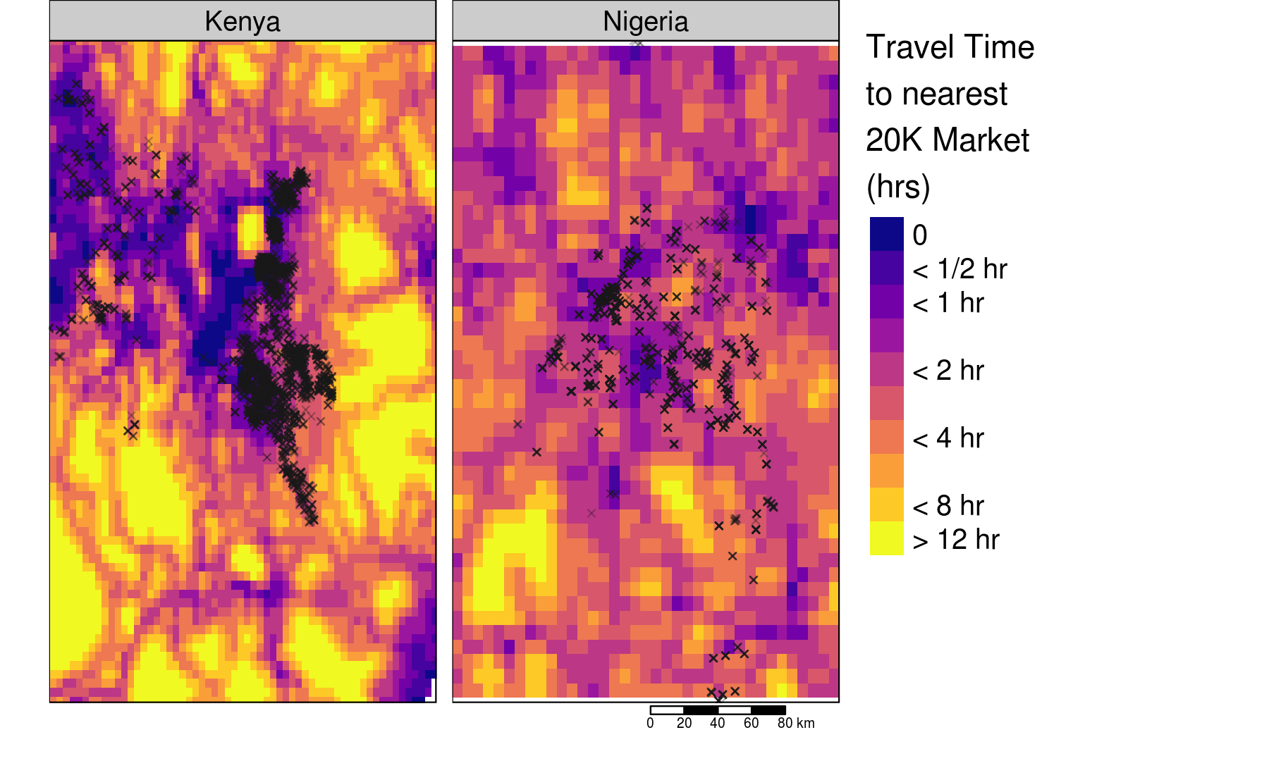
Fig. 2.13: IFPRI/HarvestChoice Travel Time to 20K Market (hrs, circa 2010)
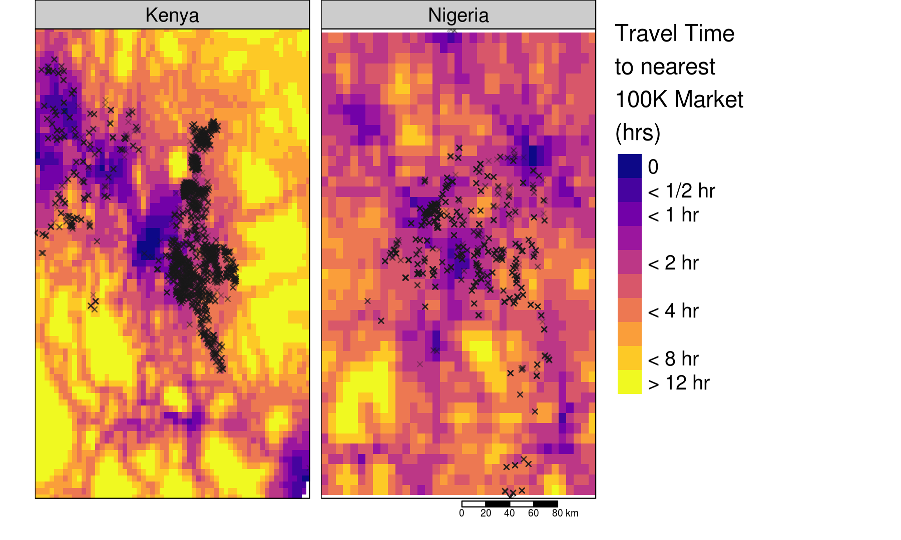
Fig. 2.14: IFPRI/HarvestChoice Travel Time to 100K Market (hrs, circa 2010)
2.4.2 CIESIN/GRUMP
Maps of roads and settlements are also available from CIESIN/GRUMP at http://sedac.ciesin.columbia.edu/data/collection/grump-v1.
Below is an example for Nigeria. Red areas are within a 5 km distance buffer to a mapped road.

NGA network
For reference there is an R geoknife and Python PyGDP library to access a subset of USGS rasters off CIDA’s THREDDS server, but currently that repository does not incorporate FEWSNET data.↩
NOAA CPC RFE Rainfall Estimates (version 2.0) for data over Africa – daily precipitation is obtained by merging GTS gauge observations and 3 kinds of satellite estimates (GPI,SSM/I and AMSU). Resolution is 0.1 degree. Units are in millimeters (mm). The RFE algorithm is based on the PingPing Xie method currently being employed as an operational product at the NOAA/Climate Prediction Center in association with USAID/FEWS-NET. Maps of daily, dekadal, and monthly rainfall estimates, as well as documentation on the RFE algorithm methodology may be found at http://www.cpc.ncep.noaa.gov/products/fews/rfe.shtml.↩
Potential Evapotranspiration – daily global PET is calculated from climate parameter data that is extracted from Global Data Assimilation System (GDAS) analysis fields. The GDAS data is generated every 6 hours by NOAA. The GDAS fields used as input to the PET calculation include air temperature, atmospheric pressure, wind speed, relative humidity, and solar radiation (long wave, short wave, outgoing and incoming). PET is computed for each 6 hour period and then summed to obtain daily totals. A day is defined as beginning at 00 hours GMT. The daily PET is calculated on a spatial basis using the Penman-Monteith equation (the formulation of Shuttleworth (1992) for reference crop evaporation is used). These equations were standardized in accordance with the FAO publication 56 for the 6-hourly calculations (Allen et al, 1998). The daily PET values are scaled up by a factor of 100 to preserve the precision to .01 mm. The PET data have a 1 deg. ground resolution and are global in spatial extent.↩
SSEBop Evapotranspiration Products (version 4) – ET is the combination of transpiration from vegetation and evaporation from soil. Actual ET (ETa) is produced using the operational SSEBop model (Senay et al., 2012) for the period 2000 to present. This model combines ET fractions generated from remotely sensed MODIS thermal imagery, acquired every 8 days, with reference ET using a thermal index approach. The unique feature of the SSEBop parameterization is that it uses pre-defined, seasonally dynamic, boundary conditions that are unique to each pixel for the “hot/dry” and “cold/wet” reference points. The actual ET data unit is millimeters (mm). The anomalies are the ratio of ETa and the corresponding median ETa, expressed as a percent value.↩
eMODIS NDVI C6 – distributed by USGS Earth Resources Observation and Science (EROS) Center. Satellite-derived vegetation products generated from the Moderate Resolution Imaging Spectroradiometer (MODIS). These products, known as eMODIS, respond to operational land monitoring applications requiring near-real time Normalized Difference Vegetation Index (NDVI) data for comparison against historical records. Real-time and historical NDVI products are composited in 10-day intervals every 5 days on a Geographic mapping grid.↩
NOAA Climate Prediction Center Africa Rainfall Climatology (version 2) – this data is a result of a project to create a satellite-estimated precipitation climatology over the Africa domain. This climatology has been created to compliment the daily operational rainfall estimate product (RFE) in order to generate anomaly fields over Africa over various timescales. In contrast to the RFE, where inputs include SSMI, AMSUB, half-hourly GPI, and GTS data, ARC uses only 3-hourly GPI and GTS data, exclusively This is due to the absence of microwave-derived estimates over a long-term historical record, and the large amount of data which makes up the operational half-hourly GPI input. As such, the ARC algorithm itself has been slightly modified in order to maintain a homogeneous and stable climate data record. GTS rain gauge data used in both static and daily-updating climatology products is of the same source, though inputs used to create GPI estimates differ slightly in source. For creation of the climatological GPI, 3-hourly Meteosat data was obtained directly from Eumetsat’s archived data group, while daily-updating products use 3-hourly data pulled from NOAA’s Meteosat data feed. Data resolution and specifications of the ARC dataset are identical to that of the RFE.↩
NOAA CPC RFE Rainfall Estimates (version 2.0) for data over Africa – daily precipitation is obtained by merging GTS gauge observations and 3 kinds of satellite estimates (GPI,SSM/I and AMSU). Resolution is 0.1 degree. Units are in millimeters (mm). The RFE algorithm is based on the PingPing Xie method currently being employed as an operational product at the NOAA/Climate Prediction Center in association with USAID/FEWS-NET. Maps of daily, dekadal, and monthly rainfall estimates, as well as documentation on the RFE algorithm methodology may be found at http://www.cpc.ncep.noaa.gov/products/fews/rfe.shtml.↩