5.2 Ghana
We use a non-hierarchical PAM (Partitioning around Medoids) clustering approach on the set of 7 variables listed below and data from Ghana GLSS6 initially (all farm households). The selected variables are defined as:
croparea_impcultivated area (in fact operated area) in ha (imputed)cropsalesvalue of sales from crops and crop byproducts (Cedis)totgrossgross household income (Cedis)totcropprodvalue of crop production (Cedis)naggross_shnon-farm income as share of total gross incomecropsales_shcrop sales as share of total crop production (in fact share of all ag products sold)aggrossgross farm income (Cedis) – not included in covariates
Note on k-mean and pam techniques: the use of means in k-means implies that clustering is highly sensitive to outliers. This can severely affects the assignment of observations to clusters. PAM (also known as k-medoids clustering) can provide a more robust algorithm in some instances.
Note on violin plots: all distributional plots below show median line in red, mean in green, and the blue region is the inferred 95% confidence interval of the mean. At present pirate plots cannot be drawn for an entire population (using weights), simple boxplots are used instead showing median and IQ range.
5.2.1 Aproach #1 – PAM Partitioning
5.2.1.1 PAM - 6 Covariates
With the selected variables (standardized) the optimal number of clusters (based on average silhouette width and total within sum of square) is 3 or 6/7. We choose to test results using k=3 and k=5 in the following run.

Fig. 3.44: PAM Clustering of GLSS6 Households (6 covariates, Euclidean Distance)
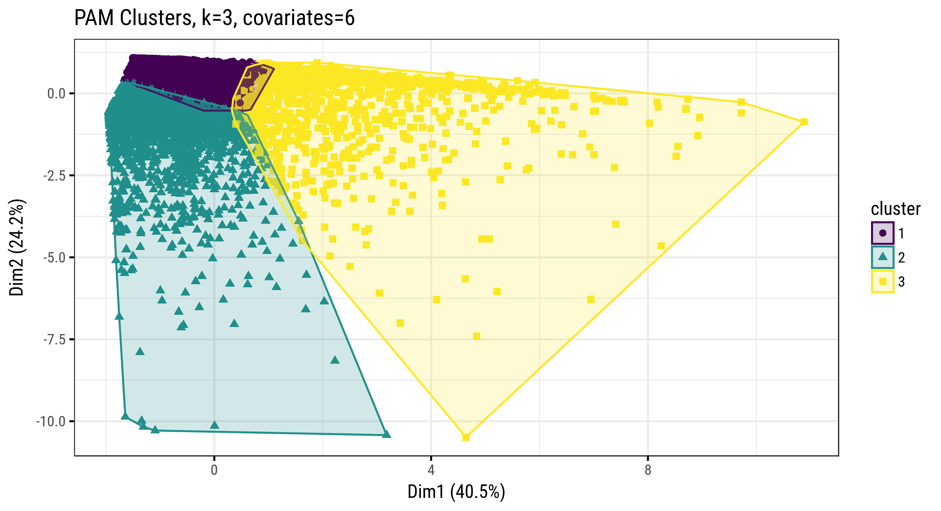
Fig. 3.45: Clusters of Farm Households (PAM, k=3, covariates=6)
The second plot shows how farm households are distributed amongst the resulting 5 clusters along our 2 axes of interest (crop sales and non-farm income).
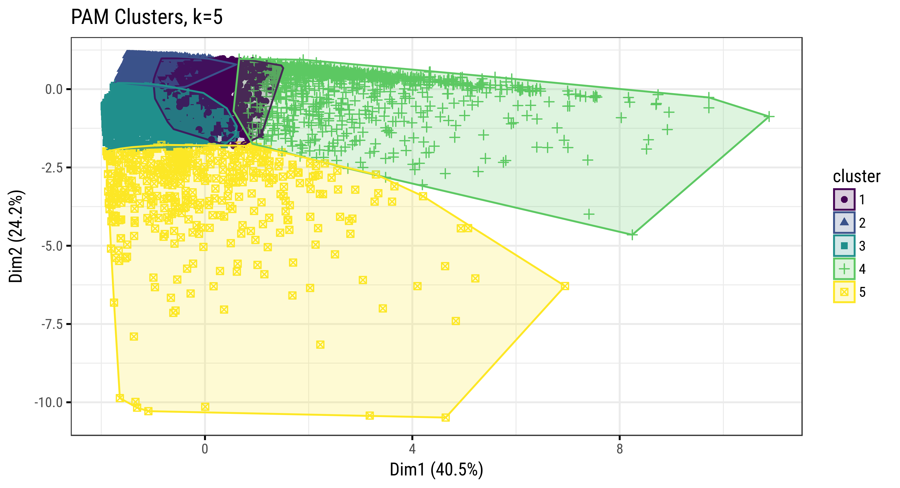
Fig. 3.46: Clusters of Farm Households (PAM, k=5, covariates=6)
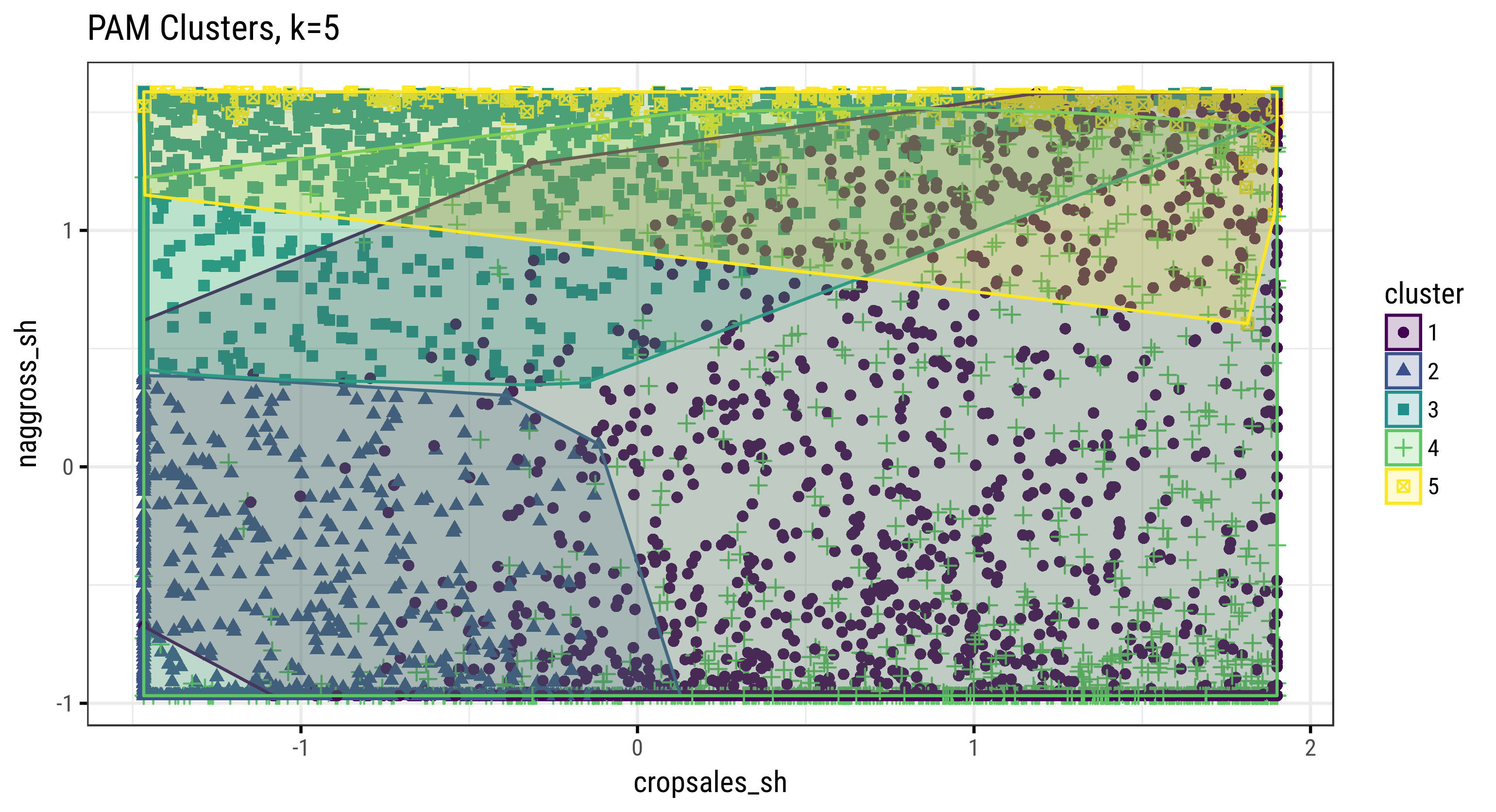
Fig. 3.46: Clusters of Farm Households (PAM, k=5, covariates=6)
Pair-wise scatter plots across all covariates (cultivated area, sales, and income variables) colored by cluster (k=5). In particular the second plot shows how the resulting 5 clusters are distributed amongst our 2 covariates of interest.
Cluster medoids (centers) are listed below for k=3 and k=5.
| croparea_imp | cropsales_sh | naggross_sh | totgross | cropsales | totcropprod |
|---|---|---|---|---|---|
| 2 | 0.4 | 0.08 | 1,159 | 200 | 849 |
| 1 | 0.3 | 0.97 | 15,345 | 120 | 458 |
| 4 | 0.7 | 0.19 | 4,297 | 2,263 | 3,322 |
| croparea_imp | cropsales_sh | naggross_sh | totgross | cropsales | totcropprod |
|---|---|---|---|---|---|
| 2 | 0.64 | 0.16 | 1,885 | 440 | 1,010 |
| 1 | 0.08 | 0.01 | 625 | 50 | 617 |
| 1 | 0.14 | 0.96 | 11,744 | 60 | 421 |
| 4 | 0.70 | 0.07 | 3,869 | 2,530 | 3,599 |
| 2 | 0.40 | 0.99 | 97,159 | 515 | 1,349 |
The violin plots below show the distribution of all 6 covariates in the sample of farm households across the resulting k=5 clusters. Actual population estimates are provided under section Key Results.
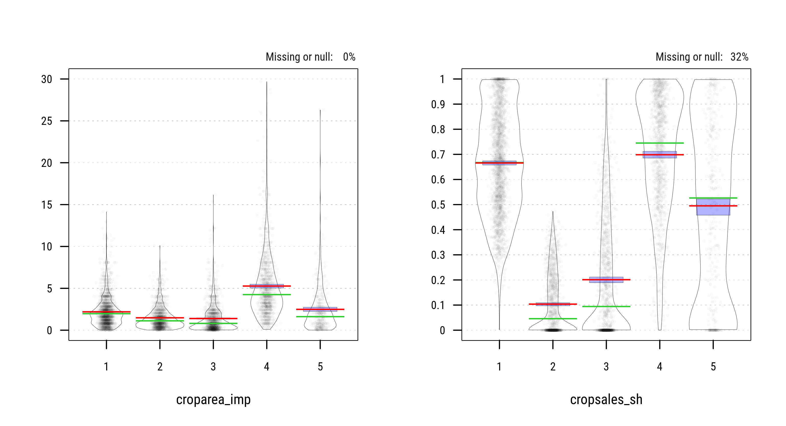
Fig. 3.47: Distribution of Household Characteristics across 5 Clusters (PAM)
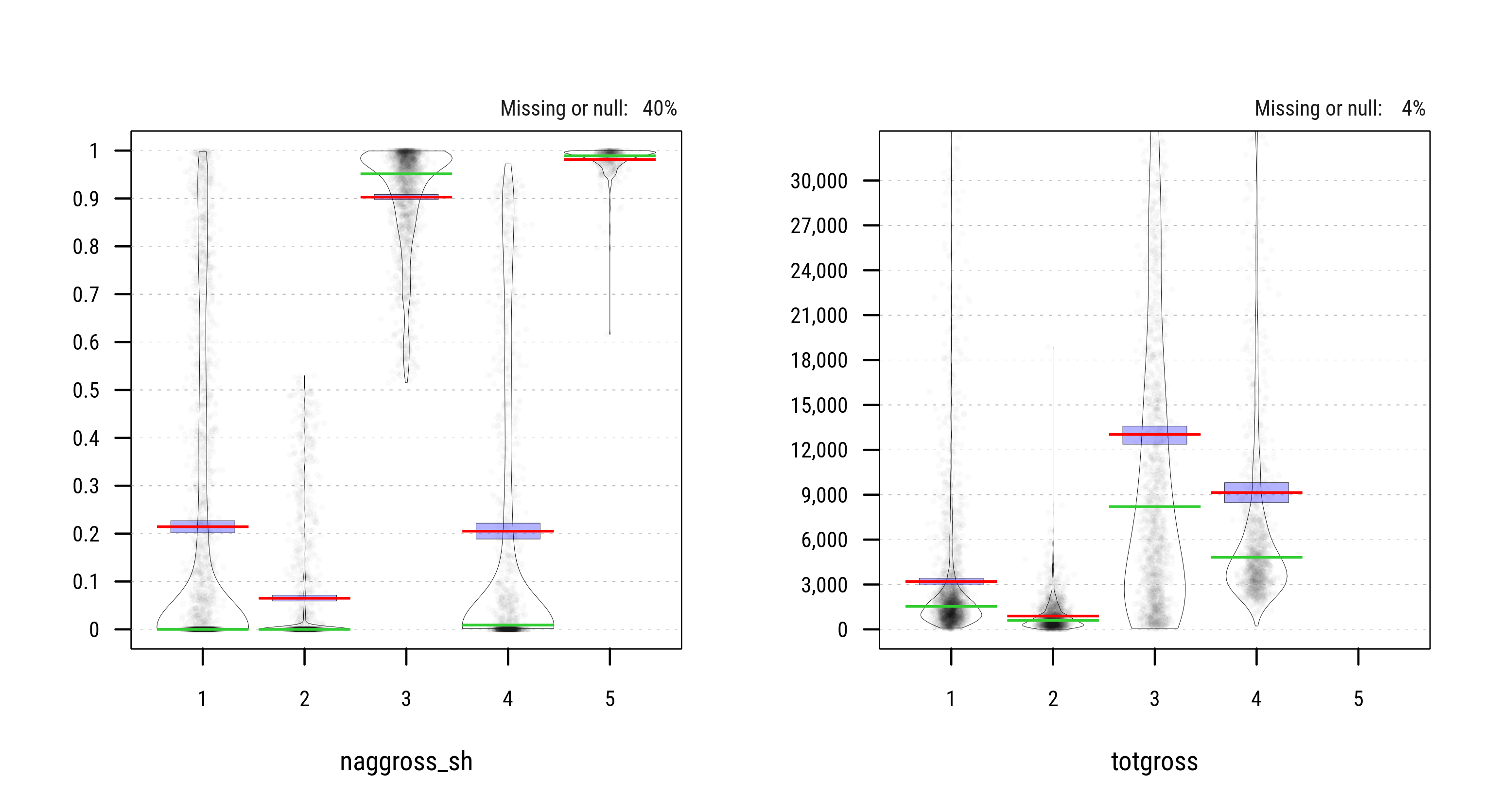
Fig. 3.47: Distribution of Household Characteristics across 5 Clusters (PAM)
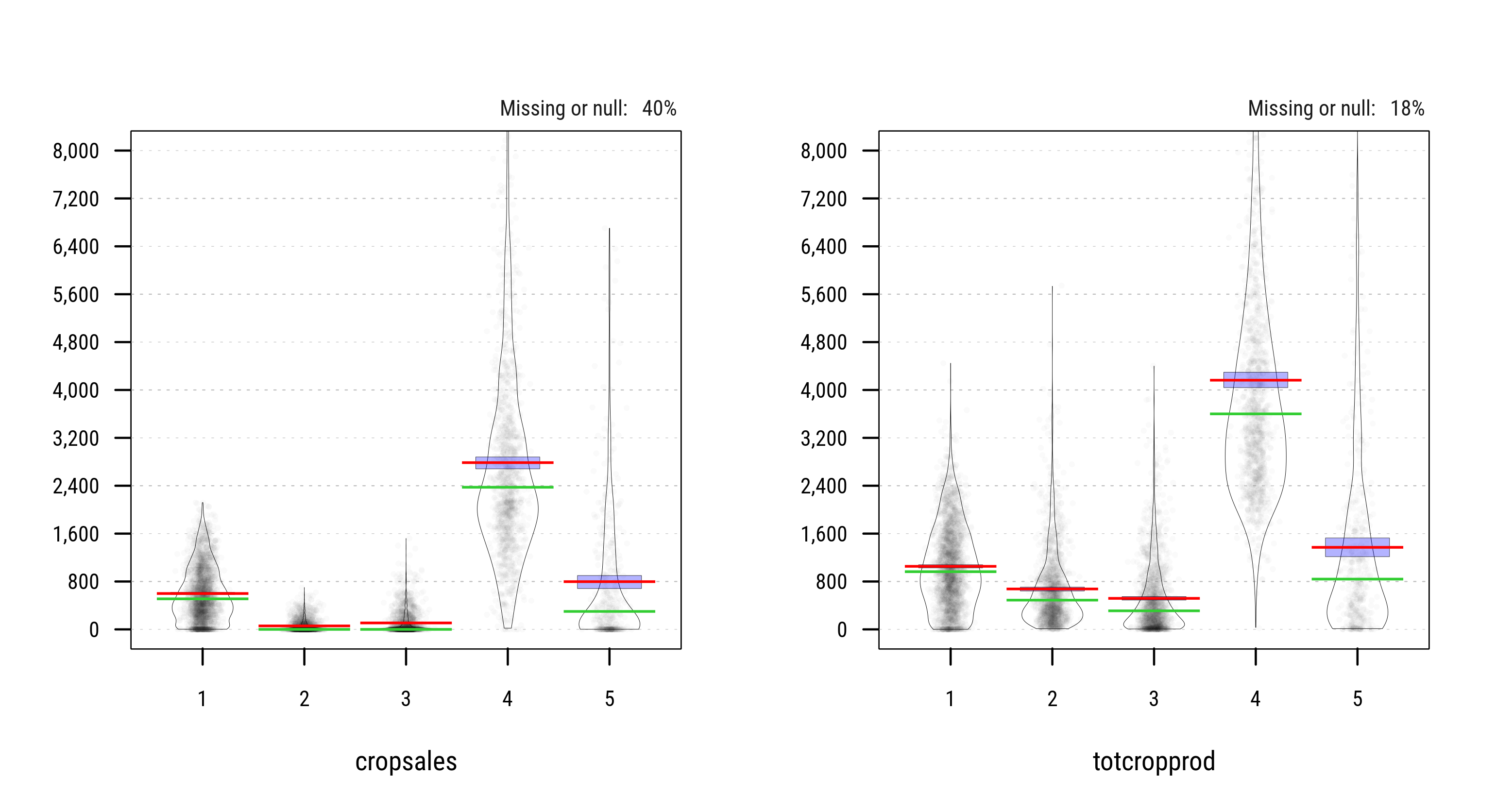
Fig. 3.47: Distribution of Household Characteristics across 5 Clusters (PAM)
5.2.1.2 PAM: 2 covariates
In the next scheme we only retain 2 covariates naggross_sh (share of non-farm income) and cropsales_sh (share of crop sales).

Fig. 3.48: PAM Clustering of GLSS6 Households (2 covariates, Euclidean Distance)
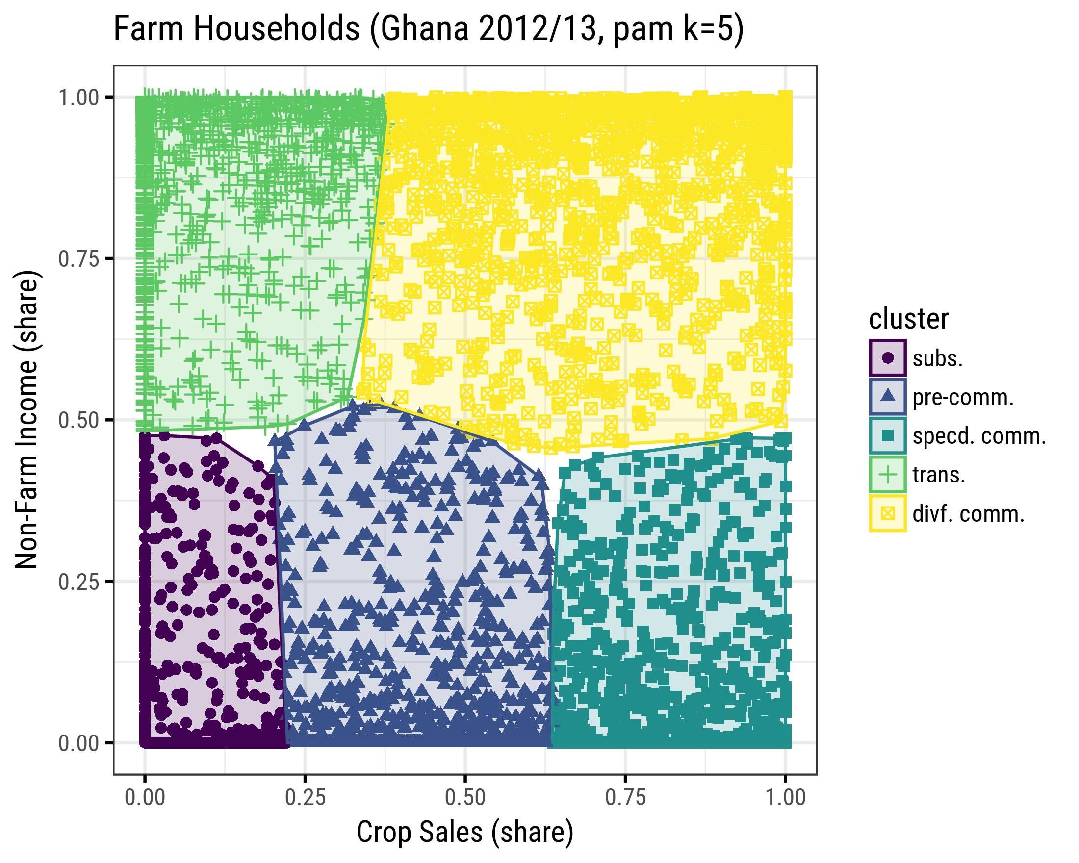
Fig. 3.49: Clusters of Farm Households (PAM, k=5, covariates=2)
Actual population statistics across the modeled 5 clusters are under section Key Results.
5.2.2 Aproach #2 – Hierarchical Clustering
[in progress, not used]
This method is sensitive to the choice of dissimilarity measure (distance matrix). Euclidean distance is often preferred, however a correlation-based distance (with similar observations sharing features that are more highly correlated) may be used to identify household profiles/preferences. Further there are multiple generic types of hierarchical clustering algorithms:
- Agglomerative – “bottom up” approach: each observation starts in its own cluster, and pairs of clusters are merged as one moves up the hierarchy (uses R
agnes()).
- Divisive – “top down” approach: all observations start in one cluster, and splits are performed recursively as one moves down the hierarchy (uses R
diana()).
- HKmean – a hybrid hierarchical k-means clustering for optimizing clustering outputs (uses R
hkmean()).
We contrast the 3 approaches, cutting the resulting trees at 5 stems.
Below are descriptive characteristics for the sample of farm households across the resulting tree branches.
5.2.3 Key Results
5.2.3.1 PAM - 6 Covariates
Below are population summaries for the selected k=5 cluster scheme.
Tables of summary statistics for the entire population. Proportions compared to manually-derived 5-class farm types.

Fig. 3.50: Est. Proportions of Farm Holdings across Clusters and Farm Types (k=5, all farm households)
| Cluster | Proportion of Farm Households | |
|---|---|---|
| clust1 | mean | 34.6 |
| CI | 32.4 - 36.8 | |
| clust2 | mean | 18.0 |
| CI | 16.3 - 19.6 | |
| clust3 | mean | 22.3 |
| CI | 20.3 - 24.3 | |
| clust4 | mean | 17.9 |
| CI | 16.0 - 19.9 | |
| clust5 | mean | 7.2 |
| CI | 6.2 - 8.2 |
Mean and median household characteristics across clusters are estimated in the tables below.
| clust1 | clust2 | clust3 | clust4 | clust5 | |||||||
|---|---|---|---|---|---|---|---|---|---|---|---|
| Variable | est. | std. err. | est. | std. err. | est. | std. err. | est. | std. err. | est. | std. err. | |
| hhsize_imp | Mean | 4.4 | 0.1 | 4.4 | 0.1 | 4.5 | 0.1 | 5.7 | 0.1 | 5.5 | 0.2 |
| Q50 | 4.0 | 0.0 | 4.0 | 0.0 | 4.0 | 0.0 | 5.0 | 0.3 | 5.0 | 0.3 | |
| agehead | Mean | 48.1 | 0.5 | 48.7 | 0.6 | 48.4 | 0.7 | 49.1 | 0.6 | 47.6 | 0.8 |
| Q50 | 45.0 | 0.3 | 47.0 | 1.3 | 47.0 | 1.0 | 47.0 | 0.8 | 45.9 | 1.0 | |
| (100 * femhead) | Mean | 21.4 | 1.4 | 29.8 | 1.7 | 37.0 | 1.9 | 9.1 | 1.1 | 19.9 | 2.3 |
| Q50 | 0.0 | 0.0 | 0.0 | 0.0 | 0.0 | 0.0 | 0.0 | 0.0 | 0.0 | 0.0 | |
| (100 * widowhead) | Mean | 4.1 | 0.7 | 6.6 | 1.0 | 5.5 | 0.8 | 1.8 | 0.5 | 3.0 | 1.1 |
| Q50 | 0.0 | 0.0 | 0.0 | 0.0 | 0.0 | 0.0 | 0.0 | 0.0 | 0.0 | 0.0 | |
| hhlabor | Mean | 2.2 | 0.0 | 2.1 | 0.1 | 2.2 | 0.1 | 2.8 | 0.1 | 2.8 | 0.1 |
| Q50 | 2.0 | 0.0 | 2.0 | 0.0 | 2.0 | 0.0 | 2.0 | 0.3 | 2.0 | 0.3 | |
| educhead | Mean | 4.2 | 0.1 | 3.3 | 0.2 | 5.1 | 0.2 | 4.5 | 0.2 | 5.7 | 0.2 |
| Q50 | 5.0 | 0.5 | 0.0 | 0.5 | 6.0 | 0.0 | 6.0 | 0.5 | 6.0 | 0.3 | |
| educave15_60 | Mean | 4.4 | 0.1 | 3.8 | 0.1 | 5.4 | 0.1 | 4.5 | 0.2 | 5.5 | 0.2 |
| Q50 | 4.8 | 0.1 | 3.7 | 0.3 | 6.0 | 0.1 | 4.8 | 0.3 | 6.0 | 0.1 | |
| educhigh | Mean | 5.9 | 0.1 | 5.4 | 0.1 | 6.9 | 0.1 | 6.5 | 0.2 | 7.6 | 0.2 |
| Q50 | 6.0 | 0.0 | 6.0 | 0.0 | 7.0 | 0.0 | 7.0 | 0.3 | 8.0 | 0.3 | |
| (100 * ownhome) | Mean | 68.7 | 1.7 | 72.3 | 2.2 | 58.5 | 2.3 | 77.4 | 1.9 | 67.0 | 4.2 |
| Q50 | 100.0 | 0.0 | 100.0 | 0.0 | 100.0 | 0.0 | 100.0 | 0.0 | 100.0 | 0.0 | |
| (100 * cellphone) | Mean | 17.9 | 1.7 | 19.2 | 1.7 | 15.1 | 1.5 | 17.9 | 2.4 | 14.3 | 2.5 |
| Q50 | 0.0 | 0.0 | 0.0 | 0.0 | 0.0 | 0.0 | 0.0 | 0.0 | 0.0 | 0.0 | |
| (100 * telephone) | Mean | 0.3 | 0.1 | 0.1 | 0.1 | 0.4 | 0.2 | 0.3 | 0.2 | 0.7 | 0.5 |
| Q50 | 0.0 | 0.0 | 0.0 | 0.0 | 0.0 | 0.0 | 0.0 | 0.0 | 0.0 | 0.0 | |
| (100 * electricity) | Mean | 38.0 | 2.6 | 28.7 | 2.6 | 53.5 | 2.6 | 40.2 | 3.3 | 57.5 | 3.6 |
| Q50 | 0.0 | 0.0 | 0.0 | 0.0 | 100.0 | 0.0 | 0.0 | 0.0 | 100.0 | 0.0 | |
| distwater | Mean | 3.3 | 1.4 | 0.7 | 0.1 | 2.2 | 0.6 | 1.0 | 0.6 | 1.4 | 0.6 |
| Q50 | 0.1 | 0.0 | 0.2 | 0.0 | 0.1 | 0.0 | 0.1 | 0.0 | 0.1 | 0.0 | |
| distroad | Mean | 0.8 | 0.2 | 1.4 | 0.3 | 0.3 | 0.1 | 0.8 | 0.2 | 0.5 | 0.2 |
| Q50 | 0.0 | 0.0 | 0.0 | 0.0 | 0.0 | 0.0 | 0.0 | 0.0 | 0.0 | 0.0 | |
| distpost | Mean | 17.5 | 1.0 | 16.9 | 0.9 | 13.1 | 0.8 | 19.0 | 1.0 | 15.5 | 1.5 |
| Q50 | 13.0 | 1.0 | 12.0 | 1.0 | 9.0 | 0.5 | 15.0 | 0.8 | 10.0 | 1.0 | |
| distbank | Mean | 15.0 | 0.8 | 14.6 | 0.8 | 10.3 | 0.6 | 16.1 | 0.9 | 11.9 | 0.9 |
| Q50 | 11.0 | 0.8 | 11.0 | 0.8 | 7.0 | 0.8 | 13.0 | 1.0 | 9.0 | 1.3 | |
| disthealth | Mean | 20.7 | 1.0 | 19.3 | 1.0 | 16.4 | 1.0 | 21.7 | 1.1 | 17.6 | 1.3 |
| Q50 | 16.0 | 0.8 | 13.0 | 1.0 | 12.0 | 1.3 | 18.0 | 1.8 | 12.0 | 1.5 | |
| clust1 | clust2 | clust3 | clust4 | clust5 | |||||||
|---|---|---|---|---|---|---|---|---|---|---|---|
| Variable | est. | std. err. | est. | std. err. | est. | std. err. | est. | std. err. | est. | std. err. | |
| croparea_imp | Mean | 2 | 0 | 1 | 0 | 1 | 0 | 5 | 0 | 3 | 0 |
| Q50 | 2 | 0 | 1 | 0 | 1 | 0 | 4 | 0 | 2 | 0 | |
| aggross | Mean | 1,366 | 67 | 786 | 38 | 524 | 33 | 4,543 | 149 | 1,834 | 209 |
| Q50 | 1,093 | 33 | 499 | 37 | 287 | 27 | 3,892 | 104 | 1,086 | 129 | |
| totgross | Mean | 3,237 | 172 | 865 | 43 | 13,281 | 624 | 9,507 | 536 | 122,868 | 5,203 |
| Q50 | 1,499 | 68 | 544 | 37 | 7,790 | 761 | 4,918 | 158 | 96,659 | 4,117 | |
| (100 * naggross_sh) | Mean | 24 | 1 | 7 | 1 | 91 | 0 | 21 | 1 | 98 | 0 |
| Q50 | 0 | 1 | 0 | 0 | 96 | 0 | 2 | 1 | 99 | 0 | |
| cropvalue | Mean | 1,018 | 29 | 652 | 32 | 458 | 30 | 4,232 | 140 | 1,358 | 112 |
| Q50 | 929 | 37 | 427 | 30 | 254 | 23 | 3,650 | 84 | 831 | 130 | |
| cropsales | Mean | 620 | 19 | 66 | 4 | 110 | 8 | 2,838 | 86 | 802 | 75 |
| Q50 | 528 | 30 | 0 | 1 | 0 | 4 | 2,448 | 76 | 301 | 65 | |
| (100 * cropsales_sh) | Mean | 69 | 1 | 11 | 1 | 21 | 1 | 70 | 1 | 52 | 2 |
| Q50 | 69 | 1 | 6 | 1 | 10 | 3 | 76 | 2 | 57 | 4 | |
| totlvstprod | Mean | 280 | 58 | 34 | 3 | 43 | 4 | 233 | 38 | 414 | 165 |
| Q50 | 10 | 5 | 0 | 0 | 0 | 0 | 25 | 7 | 3 | 4 | |
| totlivsold | Mean | 266 | 57 | 22 | 2 | 34 | 3 | 212 | 38 | 399 | 165 |
| Q50 | 0 | 0 | 0 | 0 | 0 | 0 | 0 | 3 | 0 | 0 | |
5.2.3.2 PAM - 2 Covariates
Below are population summaries for the selected k=5 cluster scheme (with only 2 covariates). First we show how farm types are distributed across small/large farm sizes (below/above 4 ha).

| Proportion of Farm Households | |||
|---|---|---|---|
| Farm Type (cluster) | \(\leq\) 4 ha | \(>\) 4 ha | |
| subs. | mean | 12.6 | 1.9 |
| CI | 11.2 - 14.0 | 1.2 - 2.6 | |
| pre-comm. | mean | 15.9 | 4.6 |
| CI | 14.3 - 17.5 | 3.7 - 5.5 | |
| specd. comm. | mean | 17.0 | 5.4 |
| CI | 15.2 - 18.9 | 4.7 - 6.2 | |
| trans. | mean | 18.8 | 2.0 |
| CI | 16.9 - 20.7 | 1.5 - 2.4 | |
| divf. comm. | mean | 17.0 | 4.6 |
| CI | 15.2 - 18.9 | 3.9 - 5.4 | |
Mean and median household characteristics across farm types are estimated below.
| subs. | pre-comm. | specd. comm. | trans. | divf. comm. | |||||||
|---|---|---|---|---|---|---|---|---|---|---|---|
| Variable | est. | std. err. | est. | std. err. | est. | std. err. | est. | std. err. | est. | std. err. | |
| hhsize_imp | Mean | 4.7 | 0.1 | 5.0 | 0.1 | 4.5 | 0.1 | 4.7 | 0.1 | 5.0 | 0.1 |
| Q50 | 4.0 | 0.3 | 5.0 | 0.3 | 4.0 | 0.0 | 4.0 | 0.3 | 5.0 | 0.3 | |
| agehead | Mean | 49.2 | 0.7 | 47.0 | 0.5 | 49.1 | 0.5 | 48.7 | 0.6 | 48.3 | 0.6 |
| Q50 | 47.0 | 1.0 | 45.0 | 0.7 | 47.0 | 0.8 | 47.0 | 1.0 | 47.0 | 0.8 | |
| (100 * femhead) | Mean | 28.3 | 1.9 | 16.0 | 1.4 | 19.3 | 1.5 | 35.2 | 1.9 | 22.9 | 1.7 |
| Q50 | 0.0 | 0.0 | 0.0 | 0.0 | 0.0 | 0.0 | 0.0 | 0.0 | 0.0 | 0.0 | |
| (100 * widowhead) | Mean | 6.0 | 1.1 | 3.9 | 0.8 | 3.5 | 0.7 | 4.6 | 0.8 | 4.3 | 0.8 |
| Q50 | 0.0 | 0.0 | 0.0 | 0.0 | 0.0 | 0.0 | 0.0 | 0.0 | 0.0 | 0.0 | |
| hhlabor | Mean | 2.2 | 0.1 | 2.4 | 0.0 | 2.2 | 0.1 | 2.3 | 0.1 | 2.5 | 0.1 |
| Q50 | 2.0 | 0.0 | 2.0 | 0.0 | 2.0 | 0.0 | 2.0 | 0.0 | 2.0 | 0.0 | |
| educhead | Mean | 3.1 | 0.2 | 3.3 | 0.1 | 4.5 | 0.1 | 5.2 | 0.2 | 5.7 | 0.2 |
| Q50 | 0.0 | 0.0 | 1.0 | 0.8 | 6.0 | 0.3 | 6.0 | 0.0 | 6.0 | 0.0 | |
| educave15_60 | Mean | 3.7 | 0.2 | 3.6 | 0.1 | 4.6 | 0.1 | 5.4 | 0.1 | 5.6 | 0.1 |
| Q50 | 3.5 | 0.3 | 3.5 | 0.3 | 5.0 | 0.3 | 6.0 | 0.1 | 6.0 | 0.0 | |
| educhigh | Mean | 5.4 | 0.2 | 5.3 | 0.1 | 6.1 | 0.1 | 7.0 | 0.1 | 7.4 | 0.1 |
| Q50 | 6.0 | 0.0 | 6.0 | 0.0 | 6.0 | 0.0 | 7.0 | 0.0 | 8.0 | 0.3 | |
| (100 * ownhome) | Mean | 73.3 | 2.4 | 73.6 | 1.8 | 73.2 | 1.7 | 60.8 | 2.1 | 62.1 | 2.7 |
| Q50 | 100.0 | 0.0 | 100.0 | 0.0 | 100.0 | 0.0 | 100.0 | 0.0 | 100.0 | 0.0 | |
| (100 * cellphone) | Mean | 22.4 | 2.0 | 19.5 | 1.9 | 16.9 | 2.0 | 16.3 | 1.7 | 13.3 | 1.6 |
| Q50 | 0.0 | 0.0 | 0.0 | 0.0 | 0.0 | 0.0 | 0.0 | 0.0 | 0.0 | 0.0 | |
| (100 * telephone) | Mean | 0.1 | 0.1 | 0.3 | 0.2 | 0.2 | 0.1 | 0.3 | 0.1 | 0.7 | 0.3 |
| Q50 | 0.0 | 0.0 | 0.0 | 0.0 | 0.0 | 0.0 | 0.0 | 0.0 | 0.0 | 0.0 | |
| (100 * electricity) | Mean | 29.5 | 2.7 | 28.8 | 2.7 | 36.6 | 2.8 | 54.1 | 2.6 | 57.8 | 3.0 |
| Q50 | 0.0 | 0.0 | 0.0 | 0.0 | 0.0 | 0.0 | 100.0 | 0.0 | 100.0 | 0.0 | |
| distwater | Mean | 0.8 | 0.2 | 2.2 | 1.1 | 2.7 | 1.3 | 2.1 | 0.6 | 2.0 | 0.7 |
| Q50 | 0.2 | 0.0 | 0.2 | 0.0 | 0.1 | 0.0 | 0.1 | 0.0 | 0.1 | 0.0 | |
| distroad | Mean | 1.6 | 0.3 | 1.1 | 0.2 | 0.8 | 0.2 | 0.4 | 0.1 | 0.3 | 0.1 |
| Q50 | 0.0 | 0.0 | 0.0 | 0.0 | 0.0 | 0.0 | 0.0 | 0.0 | 0.0 | 0.0 | |
| distpost | Mean | 18.0 | 1.0 | 19.1 | 1.0 | 18.0 | 1.2 | 12.9 | 0.8 | 14.4 | 0.8 |
| Q50 | 12.0 | 1.3 | 15.0 | 0.7 | 14.0 | 1.0 | 9.0 | 0.5 | 10.0 | 0.8 | |
| distbank | Mean | 15.2 | 1.0 | 17.1 | 0.9 | 15.3 | 1.0 | 10.0 | 0.6 | 11.7 | 0.6 |
| Q50 | 12.0 | 0.5 | 13.0 | 0.8 | 11.0 | 1.0 | 7.0 | 1.0 | 9.0 | 0.8 | |
| disthealth | Mean | 20.4 | 1.2 | 21.9 | 1.1 | 20.5 | 1.1 | 15.9 | 0.9 | 18.3 | 1.0 |
| Q50 | 15.0 | 1.3 | 16.0 | 1.1 | 17.0 | 0.8 | 11.0 | 1.3 | 15.0 | 1.0 | |
| subs. | pre-comm. | specd. comm. | trans. | divf. comm. | |||||||
|---|---|---|---|---|---|---|---|---|---|---|---|
| Variable | est. | std. err. | est. | std. err. | est. | std. err. | est. | std. err. | est. | std. err. | |
| croparea_imp | Mean | 2 | 0 | 3 | 0 | 3 | 0 | 2 | 0 | 3 | 0 |
| Q50 | 1 | 0 | 2 | 0 | 2 | 0 | 1 | 0 | 2 | 0 | |
| aggross | Mean | 1,237 | 182 | 1,912 | 93 | 2,595 | 125 | 544 | 43 | 1,767 | 106 |
| Q50 | 541 | 43 | 1,274 | 98 | 1,797 | 102 | 194 | 20 | 1,090 | 82 | |
| totgross | Mean | 1,325 | 185 | 2,063 | 100 | 2,869 | 153 | 28,426 | 2,374 | 35,485 | 1,876 |
| Q50 | 579 | 48 | 1,446 | 105 | 1,966 | 101 | 8,843 | 968 | 15,514 | 1,057 | |
| (100 * naggross_sh) | Mean | 6 | 1 | 6 | 0 | 7 | 1 | 92 | 0 | 86 | 0 |
| Q50 | 0 | 0 | 0 | 0 | 0 | 0 | 98 | 0 | 92 | 1 | |
| cropvalue | Mean | 1,096 | 180 | 1,716 | 84 | 2,123 | 82 | 535 | 43 | 1,449 | 84 |
| Q50 | 473 | 42 | 1,136 | 74 | 1,490 | 83 | 219 | 24 | 887 | 73 | |
| cropsales | Mean | 79 | 18 | 741 | 40 | 1,772 | 72 | 69 | 7 | 1,055 | 69 |
| Q50 | 0 | 0 | 429 | 26 | 1,200 | 64 | 0 | 0 | 540 | 58 | |
| (100 * cropsales_sh) | Mean | 6 | 0 | 45 | 0 | 84 | 1 | 8 | 1 | 73 | 1 |
| Q50 | 0 | 1 | 45 | 1 | 85 | 1 | 0 | 0 | 73 | 2 | |
| totlvstprod | Mean | 36 | 4 | 122 | 10 | 386 | 101 | 29 | 3 | 271 | 62 |
| Q50 | 0 | 0 | 24 | 5 | 5 | 5 | 0 | 0 | 10 | 5 | |
| totlivsold | Mean | 21 | 3 | 103 | 10 | 373 | 100 | 19 | 2 | 259 | 61 |
| Q50 | 0 | 0 | 0 | 3 | 0 | 0 | 0 | 0 | 0 | 0 | |
| subs. | pre-comm. | specd. comm. | trans. | divf. comm. | |||||||
|---|---|---|---|---|---|---|---|---|---|---|---|
| Variable | est. | std. err. | est. | std. err. | est. | std. err. | est. | std. err. | est. | std. err. | |
| (100 * seeds) | Mean | 13 | 2 | 18 | 2 | 17 | 2 | 17 | 2 | 20 | 2 |
| Q50 | 0 | 0 | 0 | 0 | 0 | 0 | 0 | 0 | 0 | 0 | |
| (100 * fert_any) | Mean | 40 | 2 | 48 | 2 | 50 | 2 | 26 | 2 | 45 | 2 |
| Q50 | 0 | 0 | 0 | 26 | 100 | 0 | 0 | 0 | 0 | 0 | |
| (100 * fert_inorg) | Mean | 32 | 2 | 37 | 2 | 35 | 2 | 20 | 2 | 30 | 2 |
| Q50 | 0 | 0 | 0 | 0 | 0 | 0 | 0 | 0 | 0 | 0 | |
| (100 * fert_org) | Mean | 10 | 1 | 13 | 2 | 17 | 2 | 8 | 1 | 17 | 2 |
| Q50 | 0 | 0 | 0 | 0 | 0 | 0 | 0 | 0 | 0 | 0 | |
| (100 * herb) | Mean | 46 | 3 | 68 | 2 | 66 | 2 | 45 | 2 | 67 | 2 |
| Q50 | 0 | 26 | 100 | 0 | 100 | 0 | 0 | 0 | 100 | 0 | |
| (100 * pest) | Mean | 17 | 2 | 33 | 2 | 43 | 3 | 19 | 2 | 42 | 2 |
| Q50 | 0 | 0 | 0 | 0 | 0 | 0 | 0 | 0 | 0 | 0 | |
| (100 * irr) | Mean | 0 | 0 | 1 | 0 | 1 | 0 | 1 | 0 | 1 | 0 |
| Q50 | 0 | 0 | 0 | 0 | 0 | 0 | 0 | 0 | 0 | 0 | |
| (100 * fuel) | Mean | 22 | 2 | 35 | 2 | 39 | 2 | 22 | 2 | 34 | 2 |
| Q50 | 0 | 0 | 0 | 0 | 0 | 0 | 0 | 0 | 0 | 0 | |
| (100 * hired_labor) | Mean | 36 | 3 | 48 | 2 | 53 | 2 | 39 | 2 | 54 | 2 |
| Q50 | 0 | 0 | 0 | 26 | 100 | 0 | 0 | 0 | 100 | 0 | |